‎

3/2 = math.exp(-math.log(2/3))
to log: log(value+1)
from log: exp(value) - 1
oldrange:0-240, new:0-100 => MinMaxScaling = (((OldValue - OldMin) * NewRange) / OldRange) + NewMin => x*100 // 240
Percentage = (Part / Total) * 100

2.1. layout resolution

x/y = 2
x*y = 440
y = sqrt(440 / 2)
x = 440 / x

2.2. model size in memory

in bf16, every parameter uses 2 bytes (in fp32 4 bytes) in addition to 8 bytes used, e.g., in the Adam optimizer https://huggingface.co/docs/transformers/perf_train_gpu_one#optimizer

7B parameter model would use (2+8)*7B=70GB
(2+8)*7*10**9/1024/1024/1024

2.3. compare two objects by features

We cannot if we don't know max and min values of features. But if we know, that min value is 0 and all max of features in the same distance from max:

import numpy as np
row1 = {'SPEAKER_00': 21.667442, 'SPEAKER_00_fuzz': 100}
row2 = {'SPEAKER_01': 7.7048755, 'SPEAKER_01_fuzz': 741}

a = np.array([[row1['SPEAKER_00'], row1['SPEAKER_00_fuzz']],
          [row2['SPEAKER_01'], row2['SPEAKER_01_fuzz']]
          ]
         )
print((a.max(axis=0) - 0))
a = a/ (a.max(axis=0) - 0)
print(a)
if np.sum(a[0] - a[1]) > 0:
    print('SPEAKER_00 has greater value')
else:
    print('SPEAKER_01 has greater value')

2.4. distance matrix

2.4.1. calc

two forms:

distance array: (distvec = pdist(x))
square form: (squareform(distvec))

from scipy.spatial.distance import pdist
from scipy.spatial.distance import squareform
import numpy as np

print(" --------- distance array:")
def cal(x, y):
    print((x- y)[0])
    return(x- y)[0]

ar = np.array([[2, 0, 2], [2, 2, 3], [-2, 4, 5], [0, 1, 9], [2, 2, 4]])

distvec = pdist(ar, metric = cal)
print()
print(distvec)
print()
print(" --------- square form:")
sqf = squareform(distvec)
print(sqf)
print()

 --------- distance array:
0
4
2
0
4
2
0
-2
-4
-2

[ 0.  4.  2.  0.  4.  2.  0. -2. -4. -2.]

 --------- square form:
[[ 0.  0.  4.  2.  0.]
 [ 0.  0.  4.  2.  0.]
 [ 4.  4.  0. -2. -4.]
 [ 2.  2. -2.  0. -2.]
 [ 0.  0. -4. -2.  0.]]

 --------- distance array:
[2 0 2] [2 2 3]
[2 0 2] [-2  4  5]
[2 0 2] [0 1 9]
[2 0 2] [2 2 4]
[2 2 3] [-2  4  5]
[2 2 3] [0 1 9]
[2 2 3] [2 2 4]
[-2  4  5] [0 1 9]
[-2  4  5] [2 2 4]
[0 1 9] [2 2 4]

[1. 1. 1. 1. 1. 1. 1. 1. 1. 1.]

 --------- square form:
[[0. 1. 1. 1. 1.]
 [1. 0. 1. 1. 1.]
 [1. 1. 0. 1. 1.]
 [1. 1. 1. 0. 1.]
 [1. 1. 1. 1. 0.]]

2.4.2. find lowest/max

import numpy as np

np.fill_diagonal(sqf, np.inf)
print("sqf\n", sqf)
# closest_points = sqf.argmin(keepdims=False) # indexes along axis=0
# print(closest_points)
i, j = np.where(sqf==sqf.min())
i, j = i[0], j[0]
print("result indexes:", i, j)
print("result:\n\t", ar[i], "\n\t", ar[j])

sqf
 [[inf  0.  4.  2.  0.]
 [ 0. inf  4.  2.  0.]
 [ 4.  4. inf -2. -4.]
 [ 2.  2. -2. inf -2.]
 [ 0.  0. -4. -2. inf]]
result indexes: 2 4
result:
	 [-2  4  5]
	 [2 2 4]

2.4.3. faster

def matrix_rand_score(a, b):
    correl = np.zeros((len(a), len(b)), dtype=float)
    for i, ac in enumerate(a):
        for j, bc in enumerate(b):
            if i > j:
                continue
            c = ac+bc
            print(i,j, c)
            correl[i, j] = c
    return correl

v = matrix_rand_score([1,2,3,4], [6,7,8,9])
print(v)

0 0 7
0 1 8
0 2 9
0 3 10
1 1 9
1 2 10
1 3 11
2 2 11
2 3 12
3 3 13
[[ 7.  8.  9. 10.]
 [ 0.  9. 10. 11.]
 [ 0.  0. 11. 12.]
 [ 0.  0.  0. 13.]]

2.5. interpolation

PolynomialFeatures - polynomial regression

create Vandermonde matrix

[[1, x_0, x_0 ** 2, x_0 ** 3, ..., x_0 ** degree]

in: y = ß0 + ß1*x + ß2*x2 + … + ßn*xn we trying to find B0, B1, B2 … Bn with linear regression

import matplotlib.pyplot as plt
from sklearn.preprocessing import PolynomialFeatures
import numpy as np
from sklearn.linear_model import Ridge

def interpol(x,y, xn):
    poly = PolynomialFeatures(degree=4, include_bias=False)
    ridge = Ridge(alpha=0.006)

    x_appr = np.linspace(x[0], xn, num=15)
    x = np.array(x).reshape(-1,1)

    # -- train
    x_poly = poly.fit_transform(x)
    ridge.fit(np.array(x_poly), y) # train

    # -- test
    x_appr_poly = poly.fit_transform(x_appr.reshape(-1,1))
    y_pred = ridge.predict(x_appr_poly) # test

    # -- plot train
    plt.scatter(x, y)

    # -- plot test
    plt.plot(x_appr, y_pred)
    plt.scatter(x_appr[-1], y_pred[-1])
    plt.ylabel("time in minutes")
    plt.title("interpolation of result for 25 max: "+ str(round(y[-1], 2)))
    # plt.savefig('./autoimgs/result_appr.png')
    plt.show()
    plt.close()
    return y_pred[-1]


x = [5,15,20]
y = [10,1260, 12175] # result
yn = interpol(x,y,xn)
print(yn)

42166.34032715159

https://scikit-learn.org/stable/auto_examples/linear_model/plot_polynomial_interpolation.html

3. common terms

feature [ˈfiːʧə]

explanatory variable in statistic or property of observation or juct column

(no term)

observation

sample

selected observations

sampling

is a selection of a subset to estimate charactersitics of the whole

variance [ˈve(ə)rɪəns]

дисперсия, разброс, результат переобучения

bias [ˈbaɪəs]

смещение, результат недообучения

pipeline [ˈpaɪplaɪn]

поэтапный процесс МЛ, используется для параметризации всего процесса

layer [ˈleɪə]

structure has input and output, part of NN

(no term)

weight [weɪt]

(no term)

end-to-end Deep Learning process -

(no term)

State-of-the-Art (SOTA) models

data ingesion

[ɪn'hiːʒən] - more broader term than ETL, is the process of connecting a wide variety of data structures into where it needs to be in a given required format and quality. to get data into any systems (storage and/or applications) that require data in a particular structure or format for operational use of the data downstream.

Stochastic

the property of being well described by a random probability distribution

latent space or latent feature space or embedding space

abstract multi-dimensional space containing feature values that we cannot interpret directly, but which encodes a meaningful internal representation of externally observed events.

in math: is an embedding of a set of items within a manifold in which items resembling each other are

positioned closer to one another in the latent space

model selection

task of choosing the best algorithm and settings of it's parameters

stratification

class percentage maintained for both training and validation sets

Degrees of freedom (df)

is the number of values in the final calculation of a statistic that are free to vary. количество «свободных» величин, необходимых для того, чтобы полностью определить вектор. может быть не только натуральным, но и любым действительным числом.

Среднеквадратическое отклонение, Standard deviation

square root of the variance

:: √( ∑(deviations of each data point from the mean) / n)

Statistical inference

is a collection of methods that deal with drawing conclusions from data that are prone to random variation.

derivative test

if function is differentiable, for finding maxima.

Probability distribution

probabilities of occurrence

independent and identically distributed i.i.d., iid, or IID

criteria that features tell something new every and was collected together that is why telling about same object y.

4. rare terms

residual [rɪˈzɪdjʊəl]: differences between observed and predicted values of data
error term: statistical error or disturbance [dɪsˈtɜːbəns] + e
Type I error: (false positive) более критична чем 2-го рода
Type II error: (false negative) понятия задач проверки статистических гипотез
fold: equal sized subsamples in cross-validation
terms of reference: техническое задание
neuron's receptive field: each neuron receives input from only a restricted area of the previous layer
Adversarial machine learning: where an attacker inputs data into a machine learning model with the aim to cause mistakes.
Coefficient of determination R^2: Его рассматривают как универсальную меру зависимости одной случайной величины от множества других. Это доля дисперсии зависимой переменной, объясняемая рассматриваемой моделью зависимости, то есть объясняющими переменными. is the proportion of the variation in the dependent variable that is predictable from the independent variable(s). Con: есть свойство, что чем больше количество независимых переменных, тем большим он становится, вносят ли дополнительные «объясняющие переменные» вклад в «объяснительную силу».
Adjusted coefficient of determination: fix con.
shrinkage [ˈSHriNGkij]: method of reduction in the effects of sampling variation.
skewness [ˈskjuːnɪs]: a measure of the asymmetry of the probability distribution of a real-valued random variable about its mean. positive - left, negative - right. 0 - no skew
Kurtosis [kəˈtəʊsɪs]: measure of the "tailedness" of the probability distribution (like skewness, but for peak). 0 -
Information content, self-information, surprisal, Shannon information: alternative way of expressing probability, quantifying the level of "surprise" of a particular outcome. odds or log-odds

5. TODO problems classification

ranking - ранжирование - Information retrieval (IR) -
- relevance score s = f(x), x=(q,d), q is a query, d is a document

Metric learning

clusterization
Dimensionality reduction снижение размерности

NLP:

Text classifiction
Word representation learning
Machine translation
NER (Named-Entity Recognizing) - classify named entities (also seeks to locate)
Information extraction
Nature Language generation
Dialogue system
Delation Learning & Knowledge Graphs
Sentiment and Emotion Analysis (sarcasm, thwarting) - classifies of emotions (positive, negative and neutral)
- speech emotion recognition (SER)
speech recognition, automatic speech recognition (ASR)
Named entity recognition
Topic modelling - descover the abstract "topic"
topic segmentation
- speaker diarization - structuring an audio stream into speaker turns
  - speaker segmentation - finding speaker change points in an audio stream
  - speaker clustering - grouping together speech segments on the basis of speaker characteristics
- Voice activity detection (VAD) is the task of detecting speech regions in a given audio stream or recording.
- Semantic Role Labeling (automatically identify actors and actions)
- Word Sense Disambiguation - Identifies which sense of a word is used in a sentence
- Keyword spotting (or word spotting) or Keyword Extraction - find instance in large data without fully recognition.
- Speech-to-text
- Text-to-speech
- relationship extraction
- Question answering
- Summarisation

Audio & Speack

ASR automatic speech recognition or Audio recognition
Keyword Spotting
Sound Event Detection
Speech Generation
Text-to-text
Human-fall detection

Computer Vision:

Image classification
Object detection - detecting instances of semantic objects of a certain class (such as humans, buildings, or cars)
Image segmentation or Semantic Segmentation - to regions, something that is more meaningful and easier to analyze
Image generation
Image retrival
Video classification
Scene graph prediction
localization
Gaze/Depth Estimation
Fine-grained recognition
person re-identification
Semantic indexing
Object Tracking
video generation
video prediction
video object segmentation
video detection
with NLP: Image captioning, Visual Qustion Answering

Data Analysis

Data Regression
Anomaly/Error
Detection…

Reinforcement Learning & Robotic

imitation learning
Robot manipulation
Locomotion
Policy Learning
Tabular's MDPs
Visual Navigation

Other Fields

Drug discovery
Disease Prediciton
Biometrical recognition
Precision Agriculture
Internet Security

5.1. Classification problem and types

binary classification (two target classes)
multi-class classification
- definition:
  - more than two exclusive targets
  - each sample can belong to only one class
- one softmax loss for all possible classes.
multi-label classification
- definition:
  - more than two non exclusive targets
  - inputs x to binary vectors y (assigning a value of 0 or 1 for each element (label) in y)
multi-class signle-label classification (more than two non exclusive targets) in which multiple target classes can be on at the same time
- One logistic regression loss for each possible class

binary: [0], [1] … n -> binary cross entropy
multi-class: [0100], [0001] … n -> categorical cross entropy
multi-label: [0101], [1110] … n -> binary cross entropy

multiclass problem is broken down into a series of binary problems using either

One-vs-One (OVO)
One-vs-Rest (OVR also called One-vs-All) OVO presents computational drawbacks, so professionals prefer the OVR approach.

Averaging techniques for metrics:

macro - compute the metric independently for each class and then take the average - treating all classes equally
weighted - weighted average for classes (score*num_occur_per_class)/totalnum
micro - aggregate the contributions of all classes to compute the average metric - micro-average is preferable if you suspect there might be class imbalance

5.2. links

https://paperswithcode.com

6. Data Analysis [ə'nælɪsɪs]

not analises

Открытый курс https://habr.com/en/company/ods/blog/327250/
Выявление скрытых зависимостей https://habr.com/en/post/339250/
example https://www.kaggle.com/startupsci/titanic-data-science-solutions
USA National institute of standards and technology (old) https://www.itl.nist.gov/div898/handbook/index.htm

Cпециалисты по анализу данных Обычно перед ними ставят задачи, которые нуждаются в уточнении формулировки, выборе метрики качества и протокола тестирования итоговой модели. Cводить задачу заказчика к формальной постановке задачи машинного обучения. Проверять качество построенной модели на исторических данных и в онлайн-эксперименте.

анализ текста и информационный поиск
коллаборативная фильтрация и рекомендательные системы
бизнес-аналитика
прогнозирование временных рядов

6.1. TODO open-source tools

FreeViz Orange 3 - exploring for teaching PSPP - free alternative for IBM SPSS Statistics - statistical analysis in social science Weka - data analysis and predictive modeling Massive Online Analysis (MOA) - large scale mining of data streams

6.2. dictionary

intrinsic dimension - for a data set - the number of variables needed in a minimal representation of the data
density -
variance - мера разброса значений случайной величины относительно её математического ожидания math#MissingReference

6.3. Steps

6.3.1. стандарт CRISP-DM или Cross-Industry Standard Process for Data Mining/Data Science

методология CRISP-DM https://en.wikipedia.org/wiki/Cross-industry_standard_process_for_data_mining

https://arxiv.org/pdf/1709.09003.pdf

2002, 2004, 2007, and 2014 show that it was the leading methodology used by industry data miners

steps:

Business Understanding
Data Understanding (EDA) - see steps in ./math#MissingReference
Data Preparation
- select data
- clean data: missing data, data errors, coding inconsistences, bad metadata
- construct data: derived attrigutes, replaced missing values
- integrate date: merge data
- format data
Modeling
- select modeling technique
- Generate Test desing: how we will test, select performance metrics
- Build Model
- Assess Model
- Reframe Setting
Evalution
Deployment

6.3.2. ASUM-DM Analytics Solutions Unified Method for Data Mining/Predictive Analytics 2015

https://developer.ibm.com/articles/architectural-thinking-in-the-wild-west-of-data-science/#asum-dm

2019 Model development process https://arxiv.org/pdf/1907.04461.pdf
IBM Data and Analytics Reference Architecture

6.3.3. Процесс разработки

методологией разработки (моделью процесса разработки) - четкие шаги

Водопадная методология (Waterfall model, «Водопад»)
- Установлены чёткие сроки окончания каждого из этапов.
- Готовый продукт передаётся заказчику только один раз в конце проекта
- где
  - отсутствует неопределённость в требованиях заказчика
  - в проектах, которые сопровождаются высокими затратами в случае провала: тщательным отслеживанием каждого из этапов и уменьшением риска допустить ошибку
- cons: слишком фиксирован, нельзя вернуться
Гибкая методология (Agile)
- cons:
  - не понятно как распределить шаги
  - циклы могут затягиваться - долго перебирают модели или подстраивают параметры
  - Документирование не регламентировано. В DS-проектах документация и история всех используемых моделей очень важна, позволяет экономить время и облегчает возможность вернуться к изначальному решению.
CIRSP-DM
- проект состоит из спринтов
- Последовательность этапов строго не определена, некоторые этапы можно менять местами. Возможна параллельность этапов (например, подготовка данных и их исследования могут вестись одновременно). Предусмотрены возвраты на предыдущие этапы.
- Фиксирование ключевых моментов проекта: графиков, найденных закономерностей, результатов проверки гипотез, используемых моделей и полученных метрик на каждой итерации цикла разработки.

6.3.4. Descriptive analytics

Проверка на нормальность - что гистограмма похожа на нормальное распределение(критерий стьюдента требует)

print(df.describe())
# Find correlations
print(applicants.corr()) # матрица корреляции
# scatter matrix Матрица рассеивания - гистограммы
from pandas.plotting import scatter_matrix
print(scatter_matrix(df))

6.3.5. Анализ временных рядов -

https://habr.com/en/post/207160/
https://machinelearningmastery.com/feature-selection-time-series-forecasting-python/
https://towardsdatascience.com/time-series-in-python-part-2-dealing-with-seasonal-data-397a65b74051
Количество записей в месяц

df['birthdate'].groupby([df.birthdate.dt.year, df.birthdate.dt.month]).agg('count')

по x - yt, по у - yt+1
- в соседние месяцы - если много на диагонали - значения продаж в соседние месяцы похожи
по x - yt, по у - yt+2
x- yt одного месяца (сумма), y - yt другого года того же месяца

Auto regressive (AR) process - when yt = c+ a1*yt-1 + a2*yt-2 …

Измерение Автокорреляция

ACF is an (complete) auto-correlation function which gives us values of auto-correlation of any series with its lagged values.
PACF is a partial auto-correlation function.

Make Stationary - remove seasonality and trend https://machinelearningmastery.com/feature-selection-time-series-forecasting-python/

from statsmodels.graphics.tsaplots import plot_acf
from matplotlib import pyplot
series = read_csv('seasonally_adjusted.csv', header=None)
plot_acf(series, lags = 150) #  lag values along the x-axis and correlation on the y-axis between -1 and 1
plot_pacf(series) # не понять. короче, то же самое, только более короткие корреляции не мешают
pyplot.show()

6.4. 2019 pro https://habr.com/ru/company/JetBrains-education/blog/438058/

https://compscicenter.ru/courses/data-mining-python/2018-spring/classes/

математическая статистика по орлу и решке определяет симметричность монетки
теория вероятности говорит, что у орла и решки одна вероятность и вероятность случайна

Регрессионный анализ:

линейный - обыкновенный
логистический

ковариация cov	корреляция corr
линейной зависимости двух случайных величин	ковариация посчитанная для стандартизованных данных
не инвариантна относительно смены масштаба	инварианта
dot(de_mean(x),de_mean(y))/(n-1), de_mean отклон от mean	cov(X,Y)/σx*σy где σ - standard deviation
Лежат между -∞ и + ∞	Лежат между -1 и +1

Оба измеряют только линейные отношения между двумя переменными, то есть когда коэффициент корреляции равен нулю, ковариация также равна нулю

6.4.1. Часть 1

1 Гистограмма
- Синонимы - строчка, объект, наблюдение
- Синонимы - стоблец, переменная, характеристика объекта, feature
Столбцы могут быть:
- количественной шкале - килограммы, секунды, доллары
- порядковой - результат бега спортсменов - 1 местов, второе, 10
- в номинальной шкале - коды или индексы чего-то
Вариационный ряд (упорядоченная выборка[1]) - полученная в результате расположения в порядке неубывания исходной последовательности независимых одинаково распределённых случайных величин. Вариационный ряд и его члены являются порядковыми статистиками.

Поря́дковые стати́стики - это упорядоченная по неубыванию выборка одинаково распределённых независимых случайных величин и её элементы, занимающие строго определенное место в ранжированной совокупности.

Квантиль Quantile - значение, которое заданная случайная величина не превышает с фиксированной вероятностью. В процентах - процентиль. «90-й процентиль массы тела у новорожденных мальчиков составляет 4 кг» - 90 % мальчиков рождаются с весом меньше, либо равным 4 кг
- First quartile - 1/4 25% - 10×(1/4) = 2.5 round up to 3 - где 10 - количество эллементов, берем 3 по возрастанию
- Second quartile 2/4 - 50%
квартиль это квантиль выраженная не в процентах а в 1/4=25 2/4=50 3/4=75

Гистограмма - количество попаданий в интервалы значений
- n_p попавших
- n_p/ (n * длинну_интервала) # площадь равна 1 - это нормирует несколько гистограм для сопоставления # приближается к плотностьи распределения при увеличении числа испытаний - которая позволяет вычислить вероятность
Kernel density estimation Ядерная оценка плотности распределения - can be ‘scott’, ‘silverman’ - задачей сглаживания данных
2
Ящиковые диаграммы (Ящики с усами (whiskers)) - min–Q1-–—Q3—max –>(толстая красная линия - медиана) - это упрощенная Гистограмма
- недостаток - скрывает горбы гистограммы
- непонятно сколько налюдений в выборках
Типичный город, чек, день на сервере
- убираем дни - которые выбросы
- если mean превышает Q3 75% - то это не очень естественно
- получается среднее арефметическое очень не устойчиво к выбросам, а медиана устойчива
Лог нормальное распределение - это распределение которое после логарифмирования становится нормальным

Медиана - число посередине выборки если ее упорядочить

Усеченное среднее - сортируем, удаляем по краям 5 или 25 и вычисл среднее арифметическое

Измерение отклонения данных
- выборочная дисперсия, на практике используют стандартное отклонение std - корень из дисперссии - корень возвращает размерность как и у исходных данных
- межквартильный размах
Доверительные интервалы - в каком интервале с точностью ~0.95 будет прогноз?
- ширина интервала будет опираться на стандартное отклонение std - больше std - шире интервал
Диаграммы рассеивания

feature - новые данные позволяющие решить задачу

кружек vs стобики -
- длины лучше
- углы норм
  - площади хуже всего
Кластеризация и иерархический класерный анализ
Кластеризация, она же
- распознавание образов без учителя
- стратификация
- таксономия
- автоматическая классификация
Инструменты
- иерархический класерный анализ
- метод к-средних - хорошо работает для больших наборов данных
- самоорганизующиеся карты Кохонена (SOM)
- Смесь (нормальных) распределений
Примеры
- разделить пользователей на группу
- выделить сегменты рынка
Классификация - два смысла
- распознавание - по известным классам
- кластеризация - по неизвестным классам
какой метод лучше - который удалось проинтерпритировать и проверить.

Типы кластеров
- плотные шаровые
- шаровые парообразные
- ленточные
- закручивающиеся
- один внутри другого
1. иерархический класерный анализ
  1. Сведение задачи к геометрической - каждый объект точка
  2. Определение меры сходства - расстояния
    - Евклидово расстояние d = sqrt((x1-y1)^2 + (x2-y2)^2)
      
      недостаток - различие по одной координате может определять расстояние
    - Квадрат Евклидова расстояния d = (x1-y1)^2 + (x2-y2)^2
      
      can be used to strengthen the effect of longer distances
      
      does not form a metric space, as it does not satisfy the triangle inequality.
    - Блок Manhettand = |x1-y1| + |x2-y2|
      
      достоинство - одной переменной тяжелее перевесить другие
  Определяется ответом на вопрос - что значит объекты похожи. Начинающим: Варда, ближайшего и среднее невзвеш.
  1. Расстояния между кластерами https://scikit-learn.org/stable/modules/clustering.html#hierarchical-clustering
    - Average linkage clustering (Среднее невзвешенное расстояние) - 3 и 4 точки - 12 расстрояний и усредняется
      
      плотные паровые скопления
    - Cetroid Method (Центроидный метод) - растояние между центрами - не показывает если одно в другом, объем не вляет
    - Complete linkage clustering (Метод дальнего соседа) - две самые далекие точки
    - Single linkage clustering (Метод ближнего соседа) - две самые близкие
      
      ленточные
    - Ward's method (Метод Варда) - хорош для k-средних
      
      плотные шаровые скопления
      
      он стремится создавать кластеры малого размера
  Для расстояния могут быть использованы собственные формулы - мера сходства сайтов по посетителям
  1. Все точки кластеры
  2. Выбираем два ближайших кластера и объединяем
  3. Остался 1 кластер
  Дендрограмма где остановиться - Дерево (5-100 записей)
  1. пронумерованные кластеры на одном расстоянии на прямой горизонтальной
  2. вертикальные линии - расстояние между кластерами в момент объединения
  3. горизонтальная - момент объединения
  Scree plot каменистая осыпь / локоть - определить число кластеров - остановиться на изломе
  - вертикаль - distance
  - горизонталь - номер слияния на равных расстояниях
    
    Участие аналитика (насколько субъективна)
  - отбор переменных
  - метод стандартизации
    - в основном два варианта - 0-1 или mean=0 std = 1
  - расстояние между кластерами
  - расстояние между объектами
  - Если кластеров нет, поцедура их все равно найдет
  Проблема ленточных кластеров
  - решение - Метод ближайшего соседа
  Недостаток иерархического анализа - хранить в оперативной памяти матрицу попарных расстояний
  - невозможность работы с гиганскими наборами данных
Метод k-means (k-средних)
Используется только евклидова метрика, другие метрики в k-медоиды
1. Задается К число кластеров и k-точек начальных кластеров
TODO 9 Прогнозирование линейно регрессией
Прогнозирование
1. есть ли тренд?
2. есть ли сезонность?
  - аддитивная - поправки не меняются от величины f = f+ g(t)
  - мультипликативные - величина добавки зависит - выступают как множители f = f*g(x)
3. Меняет ли ряд свой характер.
4. выбросы -резкие отклонения
  - отбросить
  - заменять на разумные значения
Эмпирические правила
- Если у вас меньше данных чем за 3 периода сезонных отклонений.
- Если у вас больше чем за 5 сезонных отклонений, то самые ранние данные скорее всего устарели.
Сезонная декомпозиция - ???

Пример аддитивной модели yt = a + bt + ct^2 + g(t) + εt
- a + bt + ct^2 - тренд
- εt - ошибка для каждого момента времени
- не подходит для мультипликативной сезонности
Логирифм - произведение превращает в сумму
- трюк: данные предварительно логарифмировать log(yt) = bxi+c(xi) + ε
- потенциировать - взять экспоненту и получим прогнозы для исходного ряда
Лучше не брать базой сезонов пиковый месяц
10
линейная регрессия - плохая
- 3 сезонности может
- в случае коротких временных рядов
- когда сезонности не меняются
у - номинальная шкала
- количестванная шкала (метры рубли)- регрессия
- порядковая
У - количественная
- Безопасный путь - считать что У номинальная, опасный но экономный количественный - регрессия
регрессия - weak learner

sklearn.tree.DecisionTreeClassificator - когда Y номинальной шкале

CART (Classification And Regression Tree) - и задачу распознавания и задачу регрессии решать
- используется в комбинации деревьев
- можем понять как она устроена и чему-то у них научиться
- быстро работает
Impurity Загрязнение - чтобы если толко крестики = 1 только 0 =1, а если 1/2 крестиков и 1/2 ноликов = 1/2. Варианты:
- entropy H1 = -∑pj*log2(pj)
- Gini index H2 = 1-∑pj^2=∑pj*(1-pj)
- classification error H3 = 1 - max(pj), где pj - вероятность принадлежать к классу j. на практике - доля объектов класса j в узле
Для каждой колонки перебираем пороговые значения и выбираем тот столбец с которым стало чище

Увеличение частоты узлов (насколько лучше стало после расщепления) (информативность переменных):
- ΔH = H_родителя - ( (n_левый/ n_родителя)*H_левый + (n_правый/ n_родителя)*H_правый)
- n_левый - кол-во наблюдений в левом узле
- n_родителя - кол-во наблюдений в родителе
- H_левый - загрязнение в левом потомке
- H_родителя - загрязнение которое было в родительском узле
accuracy на обучающем 90% на тестовом 72% - переобучение
TODO 11 Random Forеst, Feature selection
sklearn.tree.DecisionTreeRegressor - когда Y в количественной шкале
- лучше линейной регрессии когда у вас нелинейная зависимость ( изогнутая линия)
prune - обрезание деревьев

Деревья годятся как кирпичек

From weak to strong alg:
- stacking(5%) - X -> [Y] -> Y предсказывает основываясь на предсказаниях (предикторы)
- bagging (bootstrap aggregation) - average
- 6.19.5
Random forest - конечное решение
- 2d array, N - число строк, M - число столбцов
- случайным образом выбираем подмножество строк и столбцов - каждое дерево обучается на своем подмножестве - решает проблему декорреляции
- могут переобучаться - регулируя максимальную глубину
Параметры:
- число деревьев - сделай много, потом сокращай!
Проблемы
- декареляции - сли две выборки оказались похожи друг на друга и на выходе одно и то же - а внешне
модель сложная
- несбалансированная выборки - классы в разных пропорциях
Информативность столбцов c помощью случайных лесов:
- сложением информативностей по каждому дереву
- сравнивая out-of-bag error - берем столбце shuffle и пропускаем через дерево
Несбалансированность классов - когда 1-единичек меньше 0-ей
- решение - повторить единички
- лучшее решение - учеличить цену ошибки для 1 . class_weight = {0:.1, 1:.9} - If the class_weight doesn't sum to 1, it will basically change the regularization parameter.

6.4.2. Часть 2

4 Прогнозирование NN
1 … 12 -> 13 2 … 13 -> 14 3 … 14 -> 15

после 8, 12 наблюдения - уже не достоверно - накапливается ошибка

Чтобы это побороть тренируется две сети предсказывающие:
- одна на 1 месяц вперед
- вторая на 2 месяца вперед
В тестовую выборку нужно выбирать последние наблюдения!
- linear - регрессия
- logistic - 2 класса
- softmax - k классов
Как выделить мультипликативную сезонность? вариант
- разбиваем на окна сезонов
- скользящее среднее
- сумма сезонных поправок / кол-во наблюдений в окне = присутствует в каждом наблюдении сглаженного ряда
- исходный ряд - сглаженный = сезонные поправки
8 Факторный анализ
Факторный анализ реинкарнировался в SVD разложение - и стал полезным для рекомендательных систем

Задачи
- Cокращение числа переменных
  - входных на новые искуственные - факторы
- Измерение неизмеримого. Построение новых обобщенных показателей.
  - может оказаться, что факты измеряют исследуемую характеристику
  - исходные переменные отбирались так, чтобы косвенно имерить неизмеряемую величину
- Наглядное представление многомерных наблюдений (проецирование данных)
- Описание структуры взаимных связей между переменными, в частности выявление групп взаимозависимых переменных.
- Преодоление мультиколинеарности переменных в регрессионном анализе. Будут все ортогональны-независимы.
Коллинеарность - Если переменные линейно зависимы - то регрессионный анализ сбоит - обратную матрицу не найти - или она плохо обусловлена - маленькие изменения в обращаемой матрице приводят к большим изменениям в обращенной - что не хорошо.

Коэффициент корреляции близок к 1
7 XGBoost

Tianqi Chen

Extreme Gradient Boosting
9
Выявление структуры зависимости в данных:
- метод корреляционных плеяд - устарел
- факторный анализ - представляет модель структуры зависимости между переменных - матрица корреляции
  - Метод главных компонент - principal component analysis (PCA) (он фактически когда SVD)
  - Факторный анализ который был придуман познее - пытается воспроизвести с меьшим количеством факторов матрицу корреляции
Факторный анализ вписывается в целый подход - поиск наилучших проекций

Методы проецирования:
- Projection pursuit
- Многомерное шкалирование
- Карты Sommer'a
1 0.8 0.001

0.8 1 0.001

0.01 0.01 1

Способы:
- Если проекция целевой переменной бимодальна - то это хорошо
- В многомерном пространстве прокладываем ось в направлении максимального расброса данных - это дает сокращение размерности данных
Анализ главных компонент
- Пусть X1,X2,X3.. - cслучайный вектор
- Задача1 Найти Y=a11*X1 + a12 * X2 + … такую что D(Y) дисперсия максимальна. Y - фактор
- тогда если все axx умножить на ? то дисперсия умножиться на ? поэтому вводится дополнительное ограничение
- a1 * a1T =1 or a1^2+a1^2 + a1^2… = 1
- следующие Y - то же самое, но с новым условие corr(Y1,Y2) = 0
R - матрица ковариаций(корреляций) случайного вектора X. Задача сводится к:
- R*a = λ*a
- D(Yi)= λ
Способы завершения :
1. ∑ λ / колво первоначальных столбцов
2. отбрасываем λ у которых дисперсия меньше 1 или меньше 0.8
3. каменная осыль/ локоть
Факторный анализ который факторный анализ
- X1,X2 … - наблюдаемые переменные
- F1,F2 … - факторы ( factors, common factors) - кол-во меньше чем X
- Xi = ai1*F+ai2*F2 ….
- X = A*F + U, U = U1, U2 - то что не удалось объяснить факторами
- чем меньше дисперсия U тем лучше
```
from pandas.plotting import scatter_matrix
scatter_matrix(df)
```
Факторый анализ хорошо работает когда многие переменные коррелируют

По умолчанию работает матрица ковариации поэтому - Нужно не забыть стандартизировать.
```
from sklearn import preprocessing
scaled = preprocessing.StandardScaler().fit_transform(df)
df_scaled = pd.DataFrame(scaled, columns = df.columns)
```
sklearn.decomposition.PCA - Linear dimensionality reduction using Singular Value Decomposition of the data to project it to a lower dimensional space. The input data is centered but not scaled for each feature before applying the SVD.
```
pca = PCA(n_components = 3)
pca.fit(df_scaled)
# pca... analys here
res = pca.transfrom(df_scaled)
```
11 Калибровка классификаторов
Выход классификатора это не вероятность, а ранжировка - с какой вероятностью есть неизвестная вероятность этого класса

Калибровка это поиск вероятности для ранжировки - лучше всего на выборке валидации

calibration plot https://changhsinlee.com/python-calibration-plot/
1. Разбиваен на bins
2. x - bins, y - proportion of true outcomes
Чем больше волатильность - тем больше сомнений в качестве модели

Убрать волатильность
- isotonic регрессия
- platt метор - найти в классе логистических прямых ту, которая апроксимирует
Клссификация с нескольким количеством классов сводится к двум классам : первый против всех остальных, второй против всех остальных и тд
12 Логистическая регрессия logistic or logit regression (binary regression)
Логистическая функция от линейной комбинации - она же найрон - сеть это зависимо обучаемые ЛР c нелинейными функциями активации.

Для задачи распознавания (y 0 1)

В настоящий момент может быть лучше только в:

y = a0 + ∑a1*X , y - вероятность

конкуренты - отличаются активацией 1/(1+e^-x)
- линейная
- пробит регрессия
- логит регрессия
- Poisson regression
other
распознавание классификация инструменты
- наивный байесовский классификатор
- дискриминантный анализ
- деревья классификации
- к-го ближайшего соседа
- нейронная сеть прямого распространения
- SVM
- Случайные леса
- Gradient boosting machine
https://www.youtube.com/watch?v=VRAn1f6cUJ8

Каменистая осыпь/локоть

1	0.8	0.001
0.8	1	0.001
0.01	0.01	1

code

 # 11111111111111111
 import pandas as pd
 AH = pd.read_csv('a.csv', header=0, index_col = False)
 print(AH.head()) # header
 print(df.columns) # названия столбцов
 print(AH.shape())
 print(AH.dtypes) # типы столбцов
 print(AH.describe(inclide='all') # pre column: unique, mean, std, min, квантиль
 # Ищем аномалии!
 AH['SalePrice'].hist(bins = 60, normed=1);
 from scipy.stats.kde import gaussian_kde
 from numpy import linespace
 my_density = gaussian_kde(AH['SalePrice']) #
 x = linespace(min(AH['SalePrice']), max(AH['SalePrice']), 1)
 plot(x, my_density(x), 'g') # green line
 # смотрим на площади!ч
 # позволяет найти выбросы - отстающие пинечки
 # может быть нормальным распределением

 # 2222222222222222222222
 AH.groupby('MS Zoning')['SalePrices'].plot.hist(alpha=0.6) # несколько гистограмм на одной - НЕВАРНО - НУЖНО нормировать
 plt.legend()
 # И все равно не радует!
 # используем Ящиковую диаграмму
 ax = AH.boxplot(column='SalePrice', by='MΖ Zoning')

 print(AH['MΖ Zoning'].value_counts()) # сколько налюдений в каждой из выборок



 # диаганаль - сглаженная гистограмма, x, y - Colone, Coltwo
 #Определили самые различающиеся переменные
 df = pandas.read_csv(...)
 from pandas.plotting import scatter_matrix
 colors=('Colone': 'green', 'Coltwo': 'red')
 scatter_matrix(df,
    # размер картинки
    figsize(6,6),
    # плотность вместо гистограммы на диагонали
    diagonal='kde',
    # цвета классов
    c = df['Status'].replace(colors),
    # степень прозрачности точек
    alpha=0.2)

 # строим по определенной переменной столбцу Diagonal две гистограммы
 df.groupby('Status')['Diagonal'].plot.hist(alpha=0.6, bins=10, range=[0, 500000])
 plt.legend()

 # диаграммы рассеивания для этого же столбца
 df.plot.scatter(x='Top', y='Bottom', c=df['Status'].replace(colors))

6.5. EXAMPLES OF ANALYSIS

6.5.1. dobrinin links

https://habr.com/ru/post/204500/

Просто сравниваются 4 разных классификатора на 280 тыс. данных, разделенных 2/3, 1/3. И у всех очень низкий результат.

https://ai-news.ru/2018/08/pishem_skoringovuu_model_na_python.html https://sfeducation.ru/blog/quants/skoring_na_python

Обычный препроцессинг, классификатор случайный лес, кросс-валидация по AUC и Bagging ансамбль над лесом.

https://www.youtube.com/watch?v=q9I2ozvHOmQ

Реклама mlbootcamp.ru клона kaggle. Приз часы и футболка. На сайте нет почти ничего полезного.

http://bb3x.ru/blog/primer-resheniya-zadachi-kreditnogo-skoringa-c-podderzhkoy-svyazki-python-pandas-scikit-learn/

Копия первой ссылки https://habr.com/en/post/270201/

Очень интересная статья использующая конструирование признаков и бустинге деревьев в Microsoft Azure Machine Learning студии. Без стандартных средств pandas дело не обошлось.

6.5.2. https://github.com/firmai/industry-machine-learning

Consumer Finance

Loan Acceptance - Classification and time-series analysis for loan acceptance. ( Классический стат. анализ на выявления критичных показателй компании: бин-классификатор банкротсва SVM, Предсказание котировок ARIMA, предсказания складваются чтобы оценить рост или падение. Случайный лес бин-классификатор использется для определения важнейших показателей)
Predict Loan Repayment - Predict whether a loan will be repaid using automated feature engineering.( реклама библиотеки Featuretools для automatic feature engeering)
Loan Eligibility Ranking - System to help the banks check if a customer is eligible for a given loan. ( Отличаем выплаченные кредиты от не выплаченных. Препроцессинг с заменой на средние. Перцептрон, Случайный лес, дерево принятия решений для классификации. Результаты не проверяются и возможно переобучаются.)
Home Credit Default (FirmAI) - Predict home credit default. (Фиерические финты с Pandas, классификатор LightGBM метрика AUC, сросс-валидация StratifiedKFold. Результат это средняя feature_importance по фолдам)
Mortgage Analytics - Extensive mortgage loan analytics. (Анализ временных рядов ипотечных кредитов: проверка нулевой гипотезы, что величина является случайным блужданием; автокорреляция. Статистики: суммы; Вероятностные диаграммы; Важность по ExtraTreeClassifier; диаграммы рассеяния; матрица корреляции; уменьшение размерности методом главних компонент. Предсказание: процентной ставки, количества займов с помощью ARIMA, Linear Regression, Logistic Regression, SVM, SVR, Decision Tree, RF, k-NN. Лучшие k-NN и RandomForest.)
Credit Approval - A system for credit card approval. ( Логистическая регрессия, много анализа, 690 записей 2/3 обучающие 1/3 тестируемая. Accuracy: 0.84 gini:0.814, что довольно мало.)
Loan Risk - Predictive model to help to reduce charge-offs and losses of loans. (Apache Spark, H2O www.h2o.ai платформа для распределенного ML на Hadoop или Spark. Реализована AutoML)
Amortisation Schedule (FirmAI) - Simple amortisation schedule in python for personal use. Расчет граффика погашения. Линейная и столбчатая диаграмма.

6.6. EDA Exploratory analysis

according to CRISP: distribution of key attributes, looking for errors in the data, relationships between pairs or small numbers of attributes, results of simple aggregations, properties of significant subpopulations, and simple statistical analyses

time period
boxplot
historgram
missing values
Bivariate Exploration - impact on target: sns.violinplot

TODO https://www.kaggle.com/pavansanagapati/a-simple-tutorial-on-exploratory-data-analysis

6.6.1. types of comparison

goodness of fit - whether an observed frequency distribution differs from a theoretical distribution.
homogeneity - compares the distribution of counts for two or more groups using the same categorical variable
independence - expressed in a contingency table,

degrees of freedom (df) 1) is the number of values in the final calculation of a statistic that are free to vary. 2) number of values that are free to vary as you estimate parameters. количество «свободных» величин, необходимых для того, чтобы полностью определить вектор. может быть не только натуральным, но и любым действительным числом.

For Two Samples: df = (N1 + N2) - 2

ex: [2, 10, 11] - we estimate mean parameter, so we have: two degree

(2 + 10 + 11)/ 3 = 7.7
11 = 7.7*3 - 10 - 2

links
- https://www.statisticshowto.com/probability-and-statistics/hypothesis-testing/degrees-of-freedom/
- https://statisticsbyjim.com/hypothesis-testing/degrees-freedom-statistics/

6.6.2. skewness and kurtosis

import numpy as np
import matplotlib.pyplot as plt
from scipy.stats import kurtosis, skew

# -- toy normal distribution
mu, sigma = 0, 1 # mean and standard deviation
x = np.random.normal(mu, sigma, 1000)
# -- calc skewness and kurtosis
print( 'excess kurtosis of normal distribution (should be 0): {}'.format( kurtosis(x) ))
print( 'skewness of normal distribution (should be 0): {}'.format( skew(x) ))
# --
plt.hist(x, density=True, bins=40)  # density=False would make counts
plt.ylabel('Probability')
plt.xlabel('Data');
plt.show()

excess kurtosis of normal distribution (should be 0): -0.05048549574403838
skewness of normal distribution (should be 0): 0.2162053890291638

6.6.3. TODO normal distribution test

https://docs.scipy.org/doc/scipy/reference/generated/scipy.stats.normaltest.html

D’Agostino and Pearson’s test - 0 - means it is normal distribution

scipy.stats.normaltest(df['trip_duration_log'])

statistic - s^2 + k^2, where s is the z-score returned by skewtest and k is the z-score returned by kurtosistest.
pvalue - (p-value) A 2-sided chi squared probability for the hypothesis test. if low - there is low probability that big statistic value is realy describe not normal distribution.
- inverse is not true, not used to provide evidence for the null hypothesis.

normal distribution - symmetrical bell curve - может быть описано функцией Гауса (Gaussian distribution)

e^((−(x − μ)^2)/2*σ^2)/(σ*√2π)
- σ - standard devitation

Null Hypothesis - The null hypothesis is that the observed difference is due to chance alone. Нулевая гипотеза состоит в том, что наблюдаемая разница обусловлена только случайностью.

null distribution - when the null hypothesis is true. Here it is not normal distribution. for large number of samples equal to chi-squared distribution with two degrees of freedom.

import numpy as np
import matplotlib.pyplot as plt
from scipy.stats import normaltest

# -- toy normal distribution
mu, sigma = 0, 1 # mean and standard deviation
x = np.random.normal(mu, sigma, 100)
# -- calc skewness and kurtosis
print( 'Test whether a sample differs from a normal distribution. (should be 0): {}'.format( normaltest(x) ))

Test whether a sample differs from a normal distribution. (should be 0): NormaltestResult(statistic=4.104513172099168, pvalue=0.12844472972455415)

6.6.4. Analysis for regression model:

Linearity: assumes that the relationship between predictors and target variable is linear
No noise: eg. that there are no outliers in the data
No collinearity: if you have highly correlated predictors, it’s most likely your model will overfit
Normal distribution: more reliable predictions are made if the predictors and the target variable are normally distributed
Scale: it’s a distance-based algorithm, so preditors should be scaled — like with standard scaler

6.6.5. quartile, quantile, percentile

Range from 0 to 100
Quartiles: Range from 0 to 4.
Quantiles: Range from any value to any other value.

percentiles and quartiles are simply types of quantiles

4-quantiles are called quartiles.
5-quantiles are called quintiles.
8-quantiles are called octiles.
10-quantiles are called deciles.
100-quantiles are called percentiles.

6.7. gradient boostings vs NN

NN are very efficient for dealing with high dimensional raw data
GBM can handle missing values
GBM do not need GPU
NN big data "the more the merrier" GBM - more - bigger error

6.8. theory

types of data :

numerical - almost all values are unique
binary - only 2 values [red, blue, red, blue]
categorical - has frequent values [red, red, blue, yellow, black]

ordinal or normal

6.8.1. terms

proportions - is a mathematical statement expressing equality of two ratios a/b = c/d

6.8.2. 1 column describe

count - total count in each category of the categorical variables
среднее - mean, median,
mode - мультимодальность указывает на то, что набор данных не подчиняется нормальному распределению.
- для категориальных - count (например: 6, 2, 6, 6, 8, 9, 9, 9, 0; мода — 6 и 9).
- для числовых - пики гистограммы
- .groupby(['Outlet_Type']).agg(lambda x:x.value_counts().index[0]))
- .mode()
Measures of Dispersion
- Range - max - min
- Quartiles and Interquartile (IQR) - difference between the 3rd and the 1st quartile
- Standard Deviation - tells us how much all data points deviate from the mean value
  - .std()
- Skewness
  - skew() - data shapes are skewed or have asymmetry different from Gaussian. it is that measure.

6.8.3. categories of analysis

Descriptive analysis - What happened.
- It does this by ordering, manipulating, and interpreting raw data from various sources to turn it into valuable insights to your business.
- present our data in a meaningful way.
Exploratory analysis - How to explore data relationships.
- to find connections and generate hypotheses and solutions for specific problems
Diagnostic analysis - Why it happened.
Predictive analysis - What will happen.
Prescriptive analysis - How will it happen.

6.8.4. methods

cluster analysis - grouping a set of data elements in a way that said elements are more similar
Cohort analysis - behavioral analytics that breaks the data in a data set into related groups before analysis
- to "see patterns clearly across the life-cycle of a customer (or user), rather than slicing across all customers blindly without accounting for the natural cycle that a customer undergoes."
Regression analysis - how a dependent variable's value is affected when one (linear regression) or more independent variables (multiple regression) change or stay the same
- you can anticipate possible outcomes and make better business decisions in the future
Factor analysis - dimension reduction
Funnel analysis - analyzing a series of events that lead towards a defined goal - воронка

6.8.5. correlation

any statistical relationship between two random variables

Pearson's product-moment coefficient

sensitive only to a linear relationship between two variables

Corr(X,Y) = cov(X,Y) / σ(X)*σ(Y) = E[(X - μx)(Y-μx)]/σ(X)*σ(Y) , if σ(X)*σ(Y) > 0, E is the expected value operator.
Spearman's rank correlation

have been developed to be more robust than Pearson's, that is, more sensitive to nonlinear relationships

6.9. Feature Preparation

Ideally data is i.i.d. Independent and identically distributed - simplify computations.

get information from string columns
encoding
scaling.
- StandardScaling если нет skew.
- Если есть skew, то clipping или log scaling или нормализация.
- Если не знаем есть Skew или нет, то MinMaxScaler.
  - очень чувствителен к выбросам, поэтому их нужно обрезать
for categorical values get

6.9.1. terms

nominal features are categoricals with values that have no order
binary symmetric and asymmetric attributes - man and woman, positive results in medical is more significant than a negative
EDA - exploratory data analysis
OHE - one-hot-encoding
transformations - preserve rank of the values along each feature
- the log of the data or any other transformation of the data that preserves the order because what matters
is which ones have the smallest distance.
normalization - process of converting a variable's actual range of values into: -1 to +1, 0 to 1, the normal distribution
scaling - shifts the range of a label and/or feature value.
- linear scaling - combination of subtraction and division to replace the original value with a number
between -1 and +1 or between 0 and 1.
- logarithmic scaling
- Z-score normalization or standard scaling

6.9.2. Выбросы Outliers

quantile

https://machinelearningmastery.com/how-to-use-statistics-to-identify-outliers-in-data/

в sklearn различные скалирования по разному чувствительны к выбросам

q_low = df["col"].quantile(0.01) q_hi = df["col"].quantile(0.99) df_filtered = df[(df["col"] < q_hi) & (df["col"] > q_low)]

def outliers(p):
    df: pd.DataFrame = pd.read_pickle(p)
    # print(df.describe().to_string())
    for c in df.columns:
        q_low = df[c].quantile(0.001)
        q_hi = df[c].quantile(0.999)

        df_filtered = df[(df[c] > q_hi) | (df[c] < q_low)]
        df.drop(df_filtered.index, inplace=True)
    # print(df.describe().to_string())
    p = 'without_outliers.pickle'
    pd.to_pickle(df, p)
    print("ok")
    return p

TODO

6.9.3. IDs encoding with embaddings

6.9.4. Categorical encode

Replacing values
Encoding labels - to number 0… n_categories-1 - pandas: .get_dummies(data, drop_first=True)
One-Hot encoding - each category value into a new column and assign a 1 or 0
Binary encoding
Backward difference encoding
Miscellaneous features
MeanEncoding - A,B -> 0.7, 0.3 - mean of binary target [1,0]

Pros of MeanEncoding:

Capture information within the label, therefore rendering more predictive features
Creates a monotonic relationship between the variable and the target

Cons of MeanEncodig:

It may cause over-fitting in the model.

Label encoding

from sklearn import preprocessing
le = preprocessing.LabelEncoder()
le.fit([1, 2, 2, 6])

LabelEncoder()

le.classes_

array([1, 2, 6])

le.transform([1, 1, 2, 6])

array([0, 0, 1, 2]…)

le.inverse_transform([0, 0, 1, 2])

array([1, 1, 2, 6])

6.9.5. отбор признаков feature filtrating

Удалять:

коррелирующие переменные с целевой - только руками
значение неизменно
неважные признаки - принимают шум за сигнал, переобучаясь. Вычислительная сложность
низковариативные признаки скорее хуже, чем высоковариативные - отсекать признаки, дисперсия которых ниже определенной границы
если признаки явно бесполезны в простой модели, то не надо тянуть их и в более сложную.
Exhaustive Feature Selector

Из моего опыта - для конкретной модели - лучше всего удалить:

с низкой значимостью и коррелирующие c коррелирующие (с низкой значимостью).

6.9.6. imbalanced classes and sampling

very infrequent features are hard to learn

6.9.7. Skewed numerical feature

Linear Scaling x'=(x - x_min)/(x_max - x_min) - When the feature is more-or-less uniformly distributed across a fixed range.
Clipping if x > max, then x' = max. if x < min, then x' = min - When the feature contains some extreme outliers.
Log Scaling x' = log(x) - When the feature conforms to the power law.
Z-Score or standard scaling - When the feature distribution does not contain extreme outliers. (as Google say)

power law

is a functional relationship between two quantities

       |
     | |
     | |
     |  \
     |   \
     |    -----------------------
     |-------------------------------

6.9.8. missing values: NaN, None

pands: data.info() - количество непустых значения для каждого столбца

missing flag

for feature in df.columns: if df[feature].hasnans: df["is_" + feature + "_missing"] = np.isnull(df[feature]) * 1
Проблема выбора типичного значения
- заменить NaN на новый признак - если это отдельная группа .fillna(0)
  - Одна из хороших практик учета отсутствующих данных — генерация бинарных функций. Такие функции принимают значение 0 или 1, указывающие на то, присутствует ли в записи значение признака или оно пропущено.
- усеченная средняя - сортируем и удаляем по краям
- median - data['Age'] = data.Age.fillna(data.Age.median())
- q3-q1
- sd ?
- предсказание - лучший метод
- моды - значения которые встречаются наиболее часто
Другими распространенными практиками являются следующие подходы:
- Удаление записей с отсутствующими значениями. Обычно так делается, если число недостающих значений очень мало в сравнении со всей выборкой, при этом сам факт пропуска значения имеет случайный характер. Недостатком такой стратегии является возникновение ошибок в случаях идентичных пропусков в тестовых данных.
- Подстановка среднего, медианного или наиболее распространенного значения данного признака.
- Использование различных предсказательных моделей для прогнозирования пропущенного значения при помощи остальных данных датасета.
scikit-learn
- https://scikit-learn.org/stable/modules/impute.html
IterativeImputer
1. terms
  - impute [ɪmˈpjuːt] - приписывать
    - is to impute the missing values, i.e., to infer them from the known part of the data
  - imputation [ɪmpjʊˈteɪʃn]
  - infer [ɪnˈfɜː] - делать вывод, заключать
  Types:
  - univariate - из того столбца в котором нет
  - Multivariate - из всего набора данных
autoimpute

https://autoimpute.readthedocs.io/en/latest/

6.9.9. numerical data to bins

there might be fluctuations in those numbers that don't reflect patterns in the data, which might be noise

Новый столбец с 4 бинами возростов [0, 1, 2, 3]:

data['CatAge'] = pd.qcut(data.Age, q=4, labels=False )
data = data.drop(['Age', 'Fare'], axis=1) # удаляем оригинальыне столбцы

simple map

df['KIDSDRIV'] = df['KIDSDRIV'].map({0:0,1:1,2:2,3:2,4:2})

разложить в бины:

df['HOMEKIDS']= pd.cut(df['HOMEKIDS'],
                       bins=[0,1,2,3,4,10],
                       labels=[0,1,2,3,4],
                       include_lowest=True,
                       right=True).astype(float)

6.9.10. Sparse Classes

categorical features) are those that have very few total observations.

переобучение модели

1 большой класс и тыща супер маленьких - объединяем маленькие в большие или просто в "Others"

6.9.11. Feature engeering

Сильно зависит от модели - разные модели могут синтезировать разные операции

линейные модели - суммы столбцов создают мультиколлинеарность что мешает
neural network легко синтезирует +,-,*,counts, diff, power, rational polynominal ( bad ratio and

clusterization as a source of new features

Why?
Например два вида точек в полярных координатах и в прямоугольной системе координат
- если получается круг - то тяжелее
Когда граница пролигает по операции которую модели тяжело синтезировать
https://arxiv.org/pdf/1701.07852.pdf
- Counts ?
- Differences (diff) = x1-x2
- Logarithns (log) = log(x)
- Polynomials (poly) = 1 + 5x + 8x^2
- Powers (pow) = x^2
- Ratios = y = x1/x2
- Rational Differences (ratio_diff) y = (x1-x2)/(x3-x4)
- Rational Polynomials y = 1/(5x + 8x^2)
- Root Distance ?
- sqiare roots = sqrt(x)
- quadratic equation (quad) = y = |((-b + sqrt(b^2-4ac))/2a - (-b - sqrt(b^2-4ac))/2a)
Heaton https://towardsdatascience.com/importance-of-feature-engineering-methods-73e4c41ae5a3
NN fail at synthesizing
1. ratio_diff
2. ratio
3. quad - ?
4. log - ?
Random Forest
1. ratio_diff
2. quad
3. count
BDT Gradient Boosted Decision Trees
1. ratio_diff
2. ratio
3. counts
4. quad
Time Series
- https://machinelearningmastery.com/basic-feature-engineering-time-series-data-python/
- https://www.analyticsvidhya.com/blog/2019/12/6-powerful-feature-engineering-techniques-time-series/
- parts of date
- quarter, type of year
- logical indicator - first/last day of …
- Lag features. t-1 target value = lag . lag_1 = NaN, 1,2,3, 8…
- Rolling window - statistic based on past values - with static window size
- Expanding window feature - all past values into account
- external dataset - holidays, weather
lag correlations:
```
from statsmodels.graphics.tsaplots import plot_acf
plot_acf(data['Count'], lags=10)
plot_pacf(data['Count'], lags=10)
```
tools
1. featuretools
  1. synthetic features
    prmt=ft.list_primitives() pd.options.display.max_colwidth=150 #aggregations prmt[prmt["type"]=="aggregation"].head(10) #transformations prmt[prmt["type"]=="transform"].head(10)
2. TODO Informationsfabrik
  - https://github.com/Informationsfabrik/feature-engineering-slides/blob/master/pydata2019_feature-engineering.pdf
  - https://github.com/Informationsfabrik/feature-engineering
3. TODO TPOT
  
  https://epistasislab.github.io/tpot/
4. tsfresh - time sequence
  - https://tsfresh.readthedocs.io/en/latest/
5. ATgfe
  - https://github.com/ahmed-mohamed-sn/ATgfe
on featuretools

https://github.com/ramco-labs/automated-feature-engineering
by hands
- https://github.com/guifeliper/automated-feature-engineering/blob/master/Python/feature_engineering.py
ratio
- (A*c)/B = (A/B)*c
- (A +/- c)/B = A/B +/- c/B - the lerge c, B will have more value in ratio
- if A and B has + and - values: then A/B will sort by values with same sign and they with different.
- if A has + and - but B has only - or +, then ratio will be clearly separated for + and - of A
- if A has + and - but B has only - or +, then you can not use (-A)/B

6.9.12. Standardization, Rescale, Normalization

terms

Scale
generally means to change the range of the values

Standardize
generally means changing the values so that the distribution’s standard deviation equals one. Scaling is often implied.

Normalize (Google)
working with skew -scaling to a range, clipping, log scaling, z-score

Bucketing
reduce rare categorical

Out of Vocab (OOV)
new category for aglomerate rare categories
StandardScaler - Standardize features
Centering and scaling.
- (x-mean(x))/std(x), where x is a column
If a feature has a variance that is orders of magnitude larger than others, it might dominate the objective function and make the estimator unable to learn from other features correctly as expected.

very sensitive to the presence of outliers.

/std - it change feature importance a + b = v, do not change distribution of data -mean - do not change distribution of data. Important for PCA.

Standardization and Its Effects on K-Means Clustering Algorithm https://www.semanticscholar.org/paper/Standardization-and-Its-Effects-on-K-Means-Mohamad-Usman/1d352dd5f030589ecfe8910ab1cc0dd320bf600d?p2df
1. required by:
  - Gaussian with 0 mean and unit variance
  - objective function of a learning algorithm (such as the RBF kernel of Support Vector Machines or the L1 and
  L2 regularizers of linear models)
  - Deep learning algorithms often call for zero mean and unit variance.
  - Regression-type algorithms also benefit from normally distributed data with small sample sizes.
MinMaxScaler
- range [0, 1]
transformation:
- X_std = (X - X.min(axis=0)) / (X.max(axis=0) - X.min(axis=0))
- X_scaled = X_std * (max - min) + min
very sensitive to the presence of outliers.
MaxAbsScaler

If only positive values are present, the range is [0, 1]. If only negative values are present, the range is [-1, 0]. If both negative and positive values are present, the range is [-1, 1]

also suffers from the presence of large outliers.
RobustScaler
- [-1, 1] + outliers
transforms the feature vector by subtracting the median and then dividing by the interquartile range (75% value — 25% value).

centering and scaling statistics are based on percentiles and are therefore not influenced by a small number of very large marginal outliers.
TODO PowerTransformer, QuantileTransformer (uniform output)
Normalization

norm - функция расстояния
1. Mean normalization ( mean removal) - (-1;1)
  - data = (np.array(data) - np.mean(data)) / (max(data) - min(data))
2. Normaliztion l1 l2 (sklearn)
  works on the rows, not the columns!
  
  By default, L2 normalization is applied to each observation so the that the values in a row have a unit norm. Unit norm with L2 means that if each element were squared and summed, the total would equal 1.
  
  sklearn.preprocessing.normalize()
  - l1 - each element - ∑|x|, sum = 1
  - used with - latent semantic analysis (LSA)
Standardization (Z-score Normalization) mean removal and variance scaling (0:1)
transform the data to center and scale it by dividing non-constant features - получить нулевое матожидание(mean) и единичную дисперсию(np.std)
- mean = 0 print(np.nanmean(data, axis=0))
- std = 1 print(np.nanstd(data, axis=0))
- for line XNormed = (X - X.mean())/(X.std())
- for table XNormed = (X - X.mean(axis=0))/(X.std(axis=0))
- for table rest = (data - np.nanmean(data, axis=0))/ np.nanstd(data, axis=0)
- maintains useful information about outliers - less sensitive to them
- отнять среднне сначала или разделить - нет разницы
- numpy array with nan
from sklearn import preprocessing df = preprocessing.StandardScaler().fit_transform(df)
1. DataFrame saved with float
df /= np.nanstd(df, axis=0) df -= np.nanmean(df, axis=0)

print(df) print(df.describe()) print(df.dtypes) print(df.isna().sum().sum())

if the dataset does not have a normal or more or less normal distribution for some feature, the z-score may not be the most suitable method.
Scaling features to a range or min-max scaling or min-max normalization
- x_norm = (x - x_min)/(x_max - x_min)

6.9.13. feature selection (correlation)

Multicollinearity - one predictor variable in a multiple regression model can be perfectly predicted from the others

tech for structural risk minimization to remove redundant or irrelevant data from input

https://www.analyticsvidhya.com/blog/2016/12/introduction-to-feature-selection-methods-with-an-example-or-how-to-select-the-right-variables/

detection
detecting multicollinearity:
- The analysis exhibits the signs of multicollinearity — such as, estimates of the coefficients vary excessively from model to model.
- The t-tests for each of the individual slopes are non-significant (P > 0.05), but the overall F-test for testing all of the slopes are simultaneously 0 is significant (P < 0.05).
- The correlations among pairs of predictor variables are large.
It is possible that the pairwise correlations are small, and yet a linear dependence exists among three or even more variables.

continuous categorical

continuous Pearson LDA

categorical Anova Chi-Square
- Pearson's correlation (feature selection) is very popular for determining the relevance of all independent variables, relative to the target variable (dependent variable).
- LDA: Linear discriminant analysis is used to find a linear combination of features that characterizes or separates two or more classes (or levels) of a categorical variable.
- ANOVA: ANOVA stands for Analysis of variance. It is similar to LDA except for the fact that it is operated using one or more categorical independent features and one continuous dependent feature. It provides a statistical test of whether the means of several groups are equal or not.
- Chi-Square: It is a is a statistical test applied to the groups of categorical features to evaluate the likelihood of correlation or association between them using their frequency distribution.
questionable cause / causal fallacy / false cause

non causa pro causa ("non-cause for cause" in Latin)

correlation does not imply causation

example: "Every time I go to sleep, the sun goes down. Therefore, my going to sleep causes the sun to set."
handle correlated features
high collinearity indicates that it is exceptionally important to include all variables, as excluding any variable will cause strong confounding.
1. One way to handle multicollinear features is by performing hierarchical clustering on the Spearman rank-order correlations, picking a threshold, and keeping a single feature from each cluster
  - кластеризация для корреляций https://scikit-learn.org/stable/auto_examples/inspection/plot_permutation_importance_multicollinear.html
2. Detecting Multicollinearity Using Variance Inflation Factors.
  - https://online.stat.psu.edu/stat462/node/180/
  - https://www.datasklr.com/ols-least-squares-regression/multicollinearity
1. s
```
from statsmodels.stats.outliers_influence import variance_inflation_factor
# from statsmodels.tools.tools import add_constant
import pandas as pd

df = pd.DataFrame(
    {'a': [1, 1, 2, 3, 4],
     'b': [2, 2, 3, 2, 1],
     'c': [4, 6, 7, 8, 9],
     'd': [4, 3, 4, 5, 4]}
)

print(pd.Series([variance_inflation_factor(df.values, i) for i in
                 range(df.shape[1])], index=df.columns))
```
```
a    47.136986
b    28.931507
c    80.315068
d    40.438356
dtype: float64
```
correlation matrix

boston_pd.corr() import seaborn as sn import matplotlib.pyplot as plt corrMatrix = boston_pd.corr() sn.heatmap(corrMatrix, annot=True) plt.show()

	continuous	categorical
continuous	Pearson	LDA
categorical	Anova	Chi-Square

6.9.14. links

how to select encoding
https://machinelearningmastery.com/feature-selection-with-real-and-categorical-data/
https://scikit-learn.org/stable/modules/feature_selection.html

6.10. поиск зависимостей между признаками (Finding relationships among variables) или data mining или Интеллектуальный анализ данных

http://elib.sfu-kras.ru/bitstream/handle/2311/29014/potehin.pdf?sequence=2 https://murraylax.org/bus230/notes/relationships_print.pdf

Корреляционный анализ
Регрессинвый анализ
- Определение вклада отдельных независимых переменных
Метод последовательного сокращенияи и метод последовательного добавления параметров
NEAT for neural networks - интерпритация
кластерный анализ - если нет главного признака
Decision Tree интерпретация модели
Pattern recognition - автоматически, без привязки к бизнес логике

data mining is analysis step in "knowledge discovery in databases" KDD

6.10.1. TODO нелинейная коррелцяи - поиск через регрессию

6.10.2. simple

df.values_count(subset=['CLIENT_AGE', 'ander'], dropna=False)

6.11. Корреляционный анализ

pearson [ˈpɪsən]: standard correlation coefficient (корреляция моментов произведений)
- linear correlation between two sets of data
rank correlation (Non-parametric correlations )
1. spearman [ˈspɪəmən]: Spearman rank correlation
2. kendall [kændl]: Kendall Tau correlation coefficient

Если по меньшей мере одна из двух переменных имеет порядковую шкалу, либо не является нормально распределённой, необходимо использовать ранговую корреляцию Спирмена или τ (тау) Кендалла.

Номинальная шкала - категориальный столбец
Переменные с интервальной и с номинальной шкалой: коэффициент корреляции Пирсона (корреляция моментов произведений).
Порядковая, или ранговая, шкала - целые числа, их не имеет смысла складывать и вычитать умножать делить.

6.11.1. корреляция Пуассона

df.corr()

Свойства

r изменяется в интервале от —1 до +1.
Знак r означает, увеличивается ли одна переменная по мере того, как увеличивается другая (положительный r), или уменьшается ли одна переменная по мере того, как увеличивается другая (отрицательный r).
Величина r указывает, как близко расположены точки к прямой линии. В частности, если r = +1 или r= —1, то имеется абсолютная (функциональная) корреляция по всем точкам, лежащим на линии (практически это маловероятно); если r~0, то линейной корреляции нет (хотя может быть нелинейное соотношение). Чем ближе r к крайним точкам (±1), тем больше степень линейной связи.
Коэффициент корреляции r безразмерен, т. е. не имеет единиц измерения.
Величина r обоснована только в диапазоне значений x и y в выборке. Нельзя заключить, что он будет иметь ту же величину при рассмотрении значений x или y, которые значительно больше, чем их значения в выборке.
x и y могут взаимозаменяться, не влияя на величину r (rxy=ryx).

Расчет r может ввести в заблуждение, если:

соотношение между двумя переменными нелинейное, например квадратичное;
данные включают более одного наблюдения по каждому случаю;
есть аномальные значения (выбросы);
данные содержат ярко выраженные подгруппы наблюдений.

требования к переменным
- Обе переменные являются количественными и непрерывными
- Как минимум один из признаков (а лучше оба) имеет нормальное распределение (поэтому расчет этого коэффициента является параметрическим методом оценки взаимосвязи признаков)
- Зависимость между переменными носит линейный характер
- Гомоскедастичность (вариабельность одной переменной не зависит от значений другой переменной)
- Независимость участников исследования друг от друга (признаки Х и Y у одного участника исследования независимы от признаков Х и Y у другого)
- Парность наблюдений (признак Х и признак Y изучаются у одних и тех же участников исследования)
- Достаточно большой объем выборки
- Для адекватной проекции расчетов на генеральную совокупность выборка должна быть репрезентативной.

6.11.2. pearson vs spearman vs kendall

pearson

Each observation should have a pair of values.
Each variable should be continuous.
It should be the absence of outliers.
It assumes linearity and homoscedasticity (дисперсии одинаковы во все моменты измерения)(не рассеиваются при увеличении значений).
Corr(x,y) = ∑( (xi - mean(x))*(yi - mean(y)) ) / sqrt(∑ (xi - mean(x))^2)*sqrt(∑ (yi - mean(y))^2)

spearman and kendall

Pairs of observations are independent.
Two variables should be measured on an ordinal, interval or ratio scale.
It assumes that there is a monotonic relationship between the two variables.

Pearson correlation vs Spearman and Kendall correlation

Correlation coefficients only measure linear (Pearson) or monotonic (Spearman and Kendall) relationships.
Non-parametric correlations are less powerful because they use less information in their calculations. In the case of Pearson's correlation uses information about the mean and deviation from the mean, while non-parametric correlations use only the ordinal information and scores of pairs.

Spearman correlation vs Kendall correlation

In the normal case, Kendall correlation is more robust and efficient than Spearman correlation. It means that Kendall correlation is preferred when there are small samples or some outliers.
Kendall correlation has a O(n^2) computation complexity comparing with O(n logn) of Spearman correlation, where n is the sample size.
Spearman’s rho usually is larger than Kendall’s tau.
The interpretation of Kendall’s tau in terms of the probabilities of observing the agreeable (concordant) and non-agreeable (discordant) pairs is very direct.

6.12. Кластерный анализ

однородность и полнота

все кластеризуемые сущности были одной природы, описывались сходным набором характеристик
полнота видимо без пропусков?

иерархическая кластеризация, когда крупные кластеры дробятся на более мелкие, те в свою очередь дробятся ещё мельче, и т. д. Такие задачи называются задачами таксономии - результат дерево

6.12.1. terms

flat clusters: cluster labels [3, 3, 3, 4, 4, 4, 2, 2, 2, 1, 1, 1]
singleton clusters: with one or several point
inconsistency coefficient: the greater the difference between the objects connected by the link. for each link of linkage

6.12.2. steps

Этапы

Отбор количественных данных
Определение множества переменных, по которым будут оцениваться объекты в выборке, то есть признакового пространства.
Вычисление значений той или иной меры сходства (или различия) между объектами.
Применение метода кластерного анализа для создания групп сходных объектов.
Проверка достоверности результатов кластерного решения.

6.12.3. preparation

see 6.9

problems
- how to equaly treat all features
  - normalize all data - what about outsidders?
  - calc importance per feature
- how to choose right distance
- how to measure perfomance of clusterization
- correlation PCA with whiten=True to further remove the linear correlation across features.

weight dilema (feature weighting) (Clustering on Mixed Data Types)

the-ultimate-guide-for-clustering-mixed-data

https://medium.com/analytics-vidhya/the-ultimate-guide-for-clustering-mixed-data-1eefa0b4743b 6.8

scale each feature by dividing by standard deviation

cons: change importance of categorical features to not equal values

1. Gower dissimilarity (pip gower)

Allow to calc weight for columns.

0 (identical) and 1 (maximally dissimilar)

3 approaches:

quantitative (interval): range-normalized Manhattan distance
ordinal: variable is first ranked, then Manhattan distance is used with a special adjustment for ties
nominal: variables of k categories are first converted into k binary columns and then the Dice coefficient is used

If the data feature are categorical, then a DICE coefficient is applied. DICE is explained here. However, If you are familiar with Jaccard coefficient and or binary classification (e.g. True Positives TP and False Positives FP etc) and confusion matrices then DICE is going to be familiar as

https://github.com/Sreemanto/Gower-s-Distance/blob/master/Gower's%20Measure.ipynb

from sklearn.neighbors import DistanceMetric
import pandas as pd
import numpy as np

def gower_distance(df:pd.DataFrame):
    individual_variable_distances = []
    for c in df.columns:
        if df[c].dtype.name == 'object':
            feature_dist = DistanceMetric.get_metric('dice').pairwise(pd.get_dummies(df[c]))
        else:
            feature_dist = DistanceMetric.get_metric('manhattan').pairwise(df[[c]]) / max(np.ptp(df[c].values),1)

        # individual_variable_distances.append(feature_dist) # -- per observation (old)
        individual_variable_distances.append(np.mean(feature_dist)) # per column (new)
    # return np.array(individual_variable_distances).mean(0) # -- per observation (old)
    return np.array(individual_variable_distances) # per column (new)

# ------ main ----
df = pd.DataFrame([[1,2.6,'A'],[12,5,'X'],[4,7,'A'],[4,7,'A']])
df.columns = ['Num_1','Num_2','Cat_1']
print(df)
print([df[c].dtype.name for c in df.columns])
print("gower_distance", gower_distance(df))

v1=list("0101010101010101") # 2
v2=list("0202020202010101") # 3
v3=list("0202020212121212") # 3
df = pd.DataFrame({"v1":v1, "v2":v2, "v3":v3}) # .astype(str)
# df.v1 = df.v1.astype(int)
print(df)
print([df[c].dtype.name for c in df.columns])
# ----------- scale  -----------
# from scipy.cluster.vq import whiten
# numbers_prepared = whiten( obs = df )
gd = gower_distance(df)
print(gd)
print("this is weight")

links

2. Dimensionality Reduction

Factorial Analysis of Mixed Data (FAMD) (pip prince)

preparation:

categorical variables:
- one hot encoding
- divided by the squared root of the proportion of objects in the column (the number of 1s over the number
of observations in the column)
- subtract the mean
standard scaling for numerical.

Finally the PCA algorithm is executed on the resulting matrix to obtain the final output.

code (drop first or not? median or mean for categorical?)

import pandas as pd
import numpy as np
import math
from sklearn.decomposition import PCA

def calculate_zscore(df, columns):
  '''
  scales columns in dataframe using z-score
  '''
  df = df.copy()
  for col in columns:
      df[col] = (df[col] - df[col].mean())/df[col].std(ddof=0)

  return df


def one_hot_encode(df, columns):
  '''
  one hot encodes list of columns and
  concatenates them to the original df
  '''

  concat_df = pd.concat([pd.get_dummies(df[col], drop_first=False, prefix=col) for col in columns], axis=1)
  one_hot_cols = concat_df.columns

  return concat_df, one_hot_cols


def normalize_column_modality(df, columns):
  '''
  divides each column by the probability μₘ of the modality
  (number of ones in the column divided by N) only for one hot columns
  '''

  length = len(df)
  for col in columns:

    weight = math.sqrt(sum(df[col])/length)
    print(col, weight)
    df[col] = df[col]/weight

  return df


def center_columns(df, columns):
  '''
  center columns by subtracting the mean value
  '''
  for col in columns:
      df[col] = (df[col] - df[col].median())

  return df


def FAMD_prep(df):
  '''
  Factorial Analysis of Mixed Data (FAMD),
  which generalizes the Principal Component Analysis (PCA)
  algorithm to datasets containing numerical and categorical variables
  a) For the numerical variables
    - Standard scale (= get the z-score)

  b) For the categorical variables:
    - Get the one-hot encoded columns
    - Divide each column by the square root of its probability sqrt(μₘ)
    - Center the columns
  c) Apply a PCA algorithm over the table obtained!
  '''

  variable_distances = []

  numeric_cols = df.select_dtypes(include=np.number)
  cat_cols = df.select_dtypes(include='object')

  # numeric process
  normalized_df = calculate_zscore(df, numeric_cols)
  normalized_df = normalized_df[numeric_cols.columns]

  # categorical process
  cat_one_hot_df, one_hot_cols = one_hot_encode(df, cat_cols)
  cat_one_hot_norm_df = normalize_column_modality(cat_one_hot_df, one_hot_cols)
  cat_one_hot_norm_center_df = center_columns(cat_one_hot_norm_df, one_hot_cols)

  # Merge DataFrames
  processed_df = pd.concat([normalized_df, cat_one_hot_norm_center_df], axis=1)
  return processed_df


def FAMD_pca(df, n_components=2):
  '''
  c) Apply a PCA algorithm over the table obtained!
  '''
  # Perform (PCA)
  pca = PCA(n_components=n_components)
  principalComponents = pca.fit_transform(df)

  return principalComponents


v1=list("0101010101010101") # 2
v2=list("0202020202010101") # 3
v3=list("0202020212121212") # 3
df = pd.DataFrame({"v1":v1, "v2":v2, "v3":v3}) # .astype(str)

FAMD_processed = FAMD_prep(df)
FAMD_components = FAMD_pca(FAMD_processed, n_components=2)

print(pd.DataFrame(np.round(FAMD_components,0)))

output :session famd

from matplotlib import pyplot as plt
# print(FAMD_components)
print(pd.DataFrame(np.round(FAMD_components,0)))
plt.scatter(FAMD_components[:,0], FAMD_components[:,1])
plt.savefig('/tmp/tmp1.png')
plt.close()

from matplotlib import pyplot as plt
from scipy.cluster.hierarchy import linkage, dendrogram
l = linkage(y=FAMD_processed, method='complete', metric='matching', optimal_ordering=False)
dendrogram(Z=l, p=1.1, truncate_mode='level', labels=df.index, count_sort=False, distance_sort=False, orientation='right', leaf_font_size=15)
plt.savefig('/tmp/tmp2.png')
plt.close()

Uniform Manifold Approximation and Projection for Dimension Reduction (UMAP).

manifold learning & ideas from topological data analysis

old
- https://stats.stackexchange.com/questions/77850/assign-weights-to-variables-in-cluster-analysis
- https://stackoverflow.com/questions/6700897/how-can-i-weight-features-for-better-clustering-with-a-very-small-data-set
- https://scikit-learn.org/stable/modules/preprocessing.html
- Feature-weighted clustering with inner product induced norm based dissimilarity measures: an optimization perspective https://link.springer.com/article/10.1007/s10994-016-5623-3
- An Accurate Method of Determining Attribute Weights in Distance-Based Classification Algorithms https://www.hindawi.com/journals/mpe/2022/6936335/
- TODO: at bottom https://en.wikipedia.org/wiki/Mode_(statistics)
feature weight learning algorithm

feature weighting scheme
- distance-based clustering algorithms - limited to Euclidean, Mahalanobis, and exponential distances
  - standardize before is important
- inner product induced norm based dissimilarity measures
Dissimilarity measures are a generalized version of the distance functions

Standard deviation σ - indicates that the values tend to be close to the mean
- 2, 4, 4, 4, 5, 5, 7, 9
- mean average = 40/8 = 5
- std = sqrt(((2-5)^2 + (4-5)^2 + (4-5)^2 + (4-5)^2 …)/8) = 2
Coefficient of variation - relative standard deviation (RSD)
- ratio of the standard deviation σ to the mean μ (or its absolute value, | μ |)
- cv = σ/μ
Least absolute deviations - optimization technique for L1 norm or sum of absolute errors

least squares technique - optimization technique for minimizing the sum of the squares of the residuals

Mathematical optimization (discrete optimization) - is the selection of a best element, with regard to some criterion
- min (x^2+1) , where x ∈ R. =1, occurring at x=0
- argmax/argmin f(x) - elements of the domain of some function at which the function values are maximized/minimized.

standartization and regression
- https://stats.stackexchange.com/questions/22329/how-does-centering-the-data-get-rid-of-the-intercept-in-regression-and-pca
- https://stats.stackexchange.com/questions/19523/need-for-centering-and-standardizing-data-in-regression
PCA is a regressional model without intercept. If you forget to center your data, the 1st principal component may pierce the cloud not along the main direction of the cloud, and will be (for statistics purposes) misleading.
- Centering dont play role for clusterization but for PCA.
- unit norm required for clusterization
dimensionaly reduction, multidimensional scaling
PCA - main linear technique for dimensionality reduction. The covariance (and sometimes the correlation) matrix of the data is constructed and the eigenvectors on this matrix are computed.

Kernel PCA - nonlinear way of PCA. kernel trick.

TruncatedSVD (aka LSA) - Contrary to PCA, this estimator does not center the data before computing the singular value decomposition. This means it can work with sparse matrices efficiently.
- works on term count/tf-idf matrices (latent semantic analysis (LSA))
PCA, MCA, or t-SNE to obtain a 2 or 3 dimensional vectors for plotting.
- use t-SNE alters the scale and magnitude of the feature spaces and some methods, such as plotting centroids, will not work as shown below.
linear:
- Independent Component Analysis
- Linear Discriminant Analysis
1. Manifold learning
  approach to non-linear dimensionality reduction.
  
  Multidimensional scaling (MDS) - seeks a low-dimensional representation of the data in which the distances respect well the distances in the original high-dimensional space.
  - metric
  - non metric - preserve the order of the distances, seek for a monotonic relationship between the distances in the embedded space and the similarities/dissimilarities.
2. PCA
  recommended standard scaling
  
  step
  1. compute the covariance matrix ( Pearson correlations)
  2. Compute the eigenvectors and eigenvalues of the covariance matrix to identify the principal components
  3. Recast the Data Along the Principal Components Axes
  notes
  - Geometrically speaking, principal components represent the directions of the data that explain a maximal amount of variance
  - If the measures of correlation used are product-moment coefficients, the correlation matrix is the same as the covariance matrix of the standardized random variables X/σ(X)
  - Time complexity O(nmax^2*nmin), nmax = max(n_samples, n_features), nmin=(n_samples, n_features).
  - Memory footprint = nmax^2*nmin
3. links
  - https://en.wikipedia.org/wiki/Dimensionality_reduction
  - https://en.wikipedia.org/wiki/Eigendecomposition_of_a_matrix

normalization vs standardisation

https://www.datanovia.com/en/lessons/clustering-distance-measures/ https://iq.opengenus.org/standardization-regularization-vs-normalization/

Нужно только стандартизировать, чтобы стандартное отклонение было 1, так как это важность признака.

see 10.8.6 6.9.12.8

Normalization is useful when your data has varying scales and the algorithm you are using does not make assumptions about the distribution of your data

The goal is to make the variables comparable. Generally variables are scaled to have i) standard deviation one and ii) mean zero.

(xi - center(x))/scale(x) Where center(x) can be the mean or the median of x values, and scale(x) can be the standard deviation (SD)

https://www.analyticsvidhya.com/blog/2020/04/feature-scaling-machine-learning-normalization-standardization/

https://www.geeksforgeeks.org/normalization-vs-standardization/

Normalisation	Standardisation
min max	Mean and standard deviation is used for scaling.
Scales values between [0, 1] or [-1, 1].	It is not bounded to a certain range. (But lay in -1 1 mostly)
It is really affected by outliers.	It is much less affected by outliers.
MinMaxScaler	StandardScaler
It is useful when we don’t know about the distribution	It is useful when the feature distribution is Normal or Gaussian.

one-hot encoding

Если не сделать кодирование для категориальных столбцов, то важность будет определяться в каком значения порядке в столце

Лучше всего сделать one-hot и разделить на количесто основных значений.
как нормализация влияет на важность

Чем больше стандартное отклонение, тем тем больше значение расстояния для разных векторов и потому больше важность.

При вычислении растояния (x1 y1) (x2,y2) e = sqrt( (x1-x2)^2 + (y1-y2)^2 )

все переменные должны лежать в одном диапазоне -1 1
standardization and Euclidian distance

https://www.stat.pitt.edu/sungkyu/course/2221Fall13/lec8_mds_combined.pdf

Multidimensional scaling (MDS)

Distance, dissimilarity and similarity (or proximity)

metric - In mathematics, a distancefunction (that gives a distance between two objects)

standardized Euclidian distance - distance after standardization
overdispersion

when variance increases faster than the mean
distance
- Euclidean distance is a common measure to continuous attributes
- For multivariate data instances, distance or similarity is usually computed for each attributes and then combined.

6.12.4. Цели кластеризации

Понимание данных
- кластеров стараются сделать поменьше.
Сжатие данных. Если исходная выборка избыточно большая, то можно сократить её, оставив по одному наиболее типичному представителю от каждого кластера.
- важнее обеспечить высокую степень сходства объектов внутри каждого кластера, а кластеров может быть сколько угодно.
Обнаружение новизны (англ. novelty detection). Выделяются нетипичные объекты, которые не удаётся присоединить ни к одному из кластеров.

6.12.5. Методы кластеризации

data clustering algorithms can be of two types:

hierarchical - seeks to build a hierarchy of clusters (using a tree-like structure, called the dendrogram) following the agglomerative or the divisive approach
Partitional attempt to partition the dataset directly into a given number of clusters.

Partitional algorithms:

hard clustering, where we assign each pattern to a single cluster only
fuzzy clustering, where each pattern can belong to all the clusters with a certain membership degree (in [0, 1]) for each of them.

hierarchical, density, and similarity based

Временная сложность

Иерархический	O(n2)
k-средних, c-средних	O(nkl), где k – число кластеров, l – число итераций
Выделение связных компонент	зависит от алгоритма
Минимальное покрывающее дерево	O(n2 log n)
Послойная кластеризация	O(max(n, m)), где m < n(n-1)/2

Вероятностный подход
- K-средних и К-медиан -
  - Результат зависит от выбора исходных центров кластеров
  - Число кластеров надо знать заранее.
- Expectation–maximization algorithm
  - It is possible that it can be arbitrarily poor in high dimensions
- Алгоритмы семейства FOREL
  - Сходимость алгоритма
  - Плохая применимость алгоритма при плохой разделимости выборки на кластеры
  - зависимость от выбора начального объекта
  - Произвольное по количеству разбиение на кластеры
  - Необходимость априорных знаний о ширине (диаметре) кластеров
- Дискриминантный анализ
Neural Nenwork
- Fuzzy clustering Метод нечеткой кластеризации C-средних (C-means)
- Нейронная сеть Кохонена
- Генетический алгоритм
Логический подход. Построение дендрограммы осуществляется с помощью дерева решений.
Теоретико-графовый подход.
- Графовые алгоритмы кластеризации
  - Под дендрограммой обычно понимается дерево, построенное по матрице мер близости.
  - тер<ет наглядность при увеличении числа кластеров
Иерархический подход. - по расстоянию объединияя близкие, остановиться по Дендрограмме
DBSCAN
- does not require one to specify the number of clusters in the data a priori, as opposed to k-means.
- arbitrarily-shaped clusters. It can even find a cluster completely surrounded by (but not connected to) a different cluster
- has a notion of noise, and is robust to outliers.

moment-based approaches
spectral techniques
Elbow plots - метод локтя для определения количества кластеров в иерархическом анализе
Silhouette Scores, plot -sklearn silhouette_score() - very simular to Elbow plot and tree
- silhouette value is a measure of how similar an object is to its own cluster (cohesion) compared to other clusters (separation)
- Silhouette Samples - ?
- https://scikit-learn.org/stable/auto_examples/cluster/plot_kmeans_silhouette_analysis.html#sphx-glr-auto-examples-cluster-plot-kmeans-silhouette-analysis-py

Метод нечёткой кластеризации C-средних ( fuzzy clustering, soft k-means, c-means)

each data point can belong to more than one cluster.

6.12.6. Hierarchical clustering

https://scikit-learn.org/stable/modules/clustering.html#hierarchical-clustering

theory
https://en.wikipedia.org/wiki/Hierarchical_clustering
- linkages https://darrenho.github.io/AMA/clusteringHierarchical.pdf
hierarchical clustering [haɪərˈɑːkɪkəl] [ˈklʌstərɪŋ]
- Agglomerative: This is a "bottom-up" approach: each observation starts in its own cluster, and pairs of clusters are merged as one moves up the hierarchy.
- Divisive: This is a "top-down" approach: all observations start in one cluster, and splits are performed recursively as one moves down the hierarchy.
elbow method [ˈelbəʊ] - метод локтя affinity [əˈfɪnɪtɪ] - сходство
- euclidean [juːˈklɪdɪən] - for ward mainly
- manhattan or cityblock
- cosine
- precomputed
Linkages [ˈlɪŋkɪʤ] - связи
- Single linkage = min dij - плотные ленточные - suffer from chaining
- Complete = max dij - suffor from crowding - скученность - apoint can be closer to points in other cluster than to points in its own
- Average = sum dij / count - парообразные
- ward - minimize the within-cluster sum of squares - like k-means
  
  S C A - produces a dendrogram with no inversions - linkage distance between mergedclusters only increases as we run the algorithm
Taxonomy - close term, is a practice of categorization and classification
choosing linkage

Single and complete linkage give the same dendrogram whether you use the raw data, the log of the data or any other transformation of the data that preserves the order because what matters is which ones have the smallest distance. The other methods are sensitive to the measurement scale.
Ward distance matrix

d(u,v) = \sqrt{\frac{|v|+|s|}{T}d(v,s)^2+ \frac{|v|+|t|}{T}d(v,t)^2- \frac{|v|}{T}d(s,t)^2}

where u is the newly joined cluster consisting of clusters s and t, v is an unused cluster in the forest, T=|v|+|s|+|t|, and |*| is the cardinality of its argument. This is also known as the incremental algorithm.
choosing distance/simularity/affinity
https://www.datanovia.com/en/lessons/clustering-distance-measures/ https://en.wikipedia.org/wiki/Similarity_measure
- Евклидово расстояние d = sqrt((x1-y1)^2 + (x2-y2)^2)
  - недостаток - различие по одной координате может определять расстояние из-за возведения в квадрат
- Квадрат Евклидова расстояния d = (x1-y1)^2 + (x2-y2)^2
  - can be used to strengthen the effect of longer distances
  - does not form a metric space, as it does not satisfy the triangle inequality.
- Блок Manhettand = |x1-y1| + |x2-y2|
  - достоинство - одной переменной тяжелее перевесить другие
  - good for sparse features, or sparse noise: i.e. many of the features are zero, as in text mining using occurrences of rare words.
- Cosine simularity - −1 meaning exactly opposite, to 1 meaning exactly the same, with 0 indicating orthogonality or decorrelation
  - interesting because it is invariant to global scalings of the signal
- squared Euclidean distance - can be used to strengthen the effect of longer distances
- minkowski - d = (∑(|x1-y1|^p + |x2-y2|^p))^(1/p)
  - for p=2 equal to euclidean_distance (l2)
  - for p=1, this is equivalent to using manhattan_distance (l1)
performance
https://scikit-learn.org/stable/modules/clustering.html#clustering-performance-evaluation
1. Rand index - measures the similarity of the two assignments, ignoring permutations 0-bad 1-good
  - metrics.rand_score(labels_true, labels_pred) -does not ensure to obtain a value close to 0.0 for a random labelling
  - metrics.adjusted_rand_score(labels_true, labels_pred)
2. Mutual Information based scores -
  - metrics.adjusted_mutual_info_score(labels_true, labels_pred)
3. Homogeneity, completeness and V-measure
  - metrics.homogeneity_score(labels_true, labels_pred)
  - metrics.completeness_score(labels_true, labels_pred)
  - metrics.v_measure_score(labels_true, labels_pred)
4. Fowlkes-Mallows scores
  - metrics.fowlkes_mallows_score(labels_true, labels_pred)
5. Silhouette Coefficient [-1,1]
  - metrics.silhouette_score(X, labels, metric='euclidean')
6. Calinski-Harabasz Index
  - metrics.calinski_harabasz_score(X, labels)
  - is generally higher for convex clusters than other concepts of clusters, such as density based clusters like those obtained through DBSCAN.
  - The score is higher when clusters are dense and well separated, which relates to a standard concept of a cluster.
7. Davies-Bouldin Index
  - davies_bouldin_score(X, labels)
8. Contingency Matrix
  - from sklearn.metrics.cluster import contingency_matrix
  - contingency_matrix(x, y)
Cophenetic correlation
uses Linkage and distances

Linkage: observations or clusters (0,1), distance(2), count of collected observations in new cluster(3)

Distances:
```
[[0. 0. 2.] (1)
 [0. 0. 2.]
 [2. 2. 0.]]
```
here: [0. 0. 2.] (1) - distances between first observation and first, second, third observation

dendrogram (y - observation, x - distances) - show distance at which clusters merged

Cophenetic matrix - minimum merging distance betwen observations.

Cophenetic correlation coefficien - correlation between distance matrix and cophenetic matrix.

Measures the correlation between the distances between observations and the lowest height on the dendrogram where the points are in the same cluster.

Suppose p and q are original observations in disjoint clusters s an t, respectively and s and t are joined by a direct parent cluster u. The cophenetic distance between observations i and j is simply the distance between clusters s and t.

The correlation between the distance matrix and the cophenetic distance is one metric to help assess which clustering linkage to select.

How to use:
- It can be argued that a dendrogram is an appropriate summary of some data if the correlation between the original distances and the cophenetic distances is high.
- as the value of the Cophenetic Correlation Coefficient is quite close to 100%, we can say that the clustering is quite fit.
1. lins
2. ex
```
# Data
d0=dist(USArrests)

# Hierarchical Agglomerative Clustering
h1=hclust(d0,method='average')
h2=hclust(d0,method='complete')
h3=hclust(d0,method='ward.D')
h4=hclust(d0,method='single')

# Cophenetic Distances, for each linkage
c1=cophenetic(h1)
c2=cophenetic(h2)
c3=cophenetic(h3)
c4=cophenetic(h4)

# Correlations
cor(d0,c1) # 0.7658983
cor(d0,c2) # 0.7636926
cor(d0,c3) # 0.7553367
cor(d0,c4) # 0.5702505

# Dendograms
par(mfrow=c(2,2))
plot(h1,main='Average Linkage')
plot(h2,main='Complete Linkage')
plot(h3,main='Ward Linkage')
plot(h4,main='Single Linkage')
par(mfrow=c(1,1))
```
  We see that the correlations for average and complete are extremely similar, and their dendograms appear very similar. The correlation for ward is similar to average and complete but the dendogram looks fairly different. single linkage is doing its own thing. Best professional judgement from a subject matter expert, or precedence toward a certain link in the field of interest should probably override numeric output from cor().
sklearn
cons:
- only euclidean with Warp
- kmean and scree plot https://towardsdatascience.com/analyzing-credit-cards-kmeans-581565208cdb
- AgglomerativeClustering https://scikit-learn.org/stable/modules/generated/sklearn.cluster.AgglomerativeClustering.html#sklearn.cluster.AgglomerativeClustering
- childrens traverse https://scikit-learn.org/stable/auto_examples/cluster/plot_agglomerative_dendrogram.html#sphx-glr-auto-examples-cluster-plot-agglomerative-dendrogram-py
sklearn.cluster.AgglomerativeClustering
- labels_ - Result, each object marked with label, two clasters = [0,0,0,1,1,1]
- n_clusters_ - n cluster found
- n_leaves_ - ?
- n_connected_components_ - ?
- children_ - list of [child1, child2] for each step
- distances - list of distances from smallest, from the begining
- n_clusters - should be None
- affinity
  - "euclidean" or "l2",
  - "manhattan" or "l1" (insite affinity = 'cityblock')
  - "cosine" https://en.wikipedia.org/wiki/Cosine_similarity
  - 'precomputed'
    - sklearn.metrics.pairwise_distances
      
      'cityblock' metrics.pairwise.manhattan_distances
      
      'cosine' metrics.pairwise.cosine_distances
      
      'euclidean' metrics.pairwise.euclidean_distances
      
      'haversine' metrics.pairwise.haversine_distances
      
      'l1' metrics.pairwise.manhattan_distances
      
      'l2' metrics.pairwise.euclidean_distances
      
      'manhattan' metrics.pairwise.manhattan_distances
      
      'nan_euclidean' metrics.pairwise.nan_euclidean_distances

scipy

pdist defaults: metric='euclidean'
linkage defaults: method='single', metric='euclidean'

https://www.youtube.com/watch?v=l4vTwXL_5Cc

from sklearn import cluster, datasets
n_samples = 1500
noisy_circles = datasets.make_circles(n_samples=n_samples, factor=0.5, noise=0.05)
X = noisy_circles

from scipy.spatial.distance import pdist
distances = pdist(X, 'euclidean')
print(Y)
Y = linkage(distances)
print(Y)

6.12.7. Automatic clustering

k-means
def
- стремится минимизировать саммарное квадратичное отклонение точек кластеров от центров этих кластеров
- observations to those clusters so that the means across clusters (for all variables) are as different from each other as possible.
- assigning examples to clusters to maximize the differences in means for continuous variables
cons
- только евклидово расстрояние
- решение зависит от начальных центров
- надо определять число кластеров
- слишком много вычислений расстояний
- на поздних итерациях мало точек меняют кластер
- Не гарантируется достижение глобального минимума суммарного квадратичного отклонения V, а только одного из локальных минимумов.
- ищет только шаровые скопления
Альтернативы
- Gaussian mixture model
EM clustering - expectation maximization
Предполагается что исходные данные можно представить в виде гауссовского распределения.

EM algorithm attempts to approximate the observed distributions of values based on mixtures of different distributions in different clusters

EM для:
- для разделения смеси гауссиан.
- используется для оценки максимального правдоподобия при вычислении параметров статистической модели со скрытыми переменными.
  - распределение помогает понять, сколько человек, сдающих экзамен, получат ту или иную оценку.
  - правдоподобие - это вероятность того, что кривая нормального распределения с оцененными значениями среднего арифметического и дисперсии будет достаточно точно описывать (?)
    - На основании этих оцененных параметров модели считается гипотетическая вероятность появления того или иного исхода, называемая правдоподобием
  - вероятность - Шанс, что мы пронаблюдаем определенные оценки с определенной частотой
How
- Describe each cluster by its centroid (mean), covariance (so that we can have elliptical clusters), and weight
(the size of the cluster).
- The probability that a point belongs to a cluster is now given by a multivariate Gaussian probability distribution (multivariate - depending on multiple variables).
pros:
- clusters that are overlapping, or ones that are not of circular shape
- “soft clustering” - one point have distribution of probabilities over clusters
cons:
- maximum may be local, so we can run the algorithm several times to get better clusters.
two steps:
1. E-step - calculating, for each point, the probabilities of it belonging to each of the current clusters (which, again, may be randomly created at the beginning)
2. M-step - recalculates the parameters of each cluster, using the assignments of points to the previous set of clusters.
3. Предыдущие два шага повторяются до тех пор, пока параметры модели и кластерное распределение не уравняются.
недостатки:
- С ростом количества итераций падает производительность алгоритма.
- EM не всегда находит оптимальные параметры и может застрять в локальном оптимуме, так и не найдя глобальный.
Mixture model - Гауссова Смесь Распределений
1. sklearn: GaussianMixture
  https://cmdlinetips.com/2021/03/gaussian-mixture-models-with-scikit-learn-in-python/
  
  Информационный критерий Акаике (AIC) Akaike information criterion - Чем меньше тем лучше AIC = 2k-2ln(L)
  - k - число параметров в статистической модели
  - L — максимизированное значение функции правдоподобия модели.
  Bayesian information criterion (BIC) - налагает больший штраф на увеличение количества параметров по сравнению с AIC BIC = kln(n)-2l n - обхем выборки
AffinityPropagation
TODO NN Semantic Clustering by Adopting Nearest neighbors (SCAN)

https://arxiv.org/abs/2005.12320

6.12.8. mistakes

Lack of an exhaustive Exploratory Data Analysis (EDA) and digestible Data Cleaning. how they correlate with each other are essential. WHY you decided to choose the respective approach.

6.12.9. quality, validation, evalutaion

arror rate, accuracy
confusion matrix:

actual P(1) actua N(0)

out P(1) TP FP

out N(0) FN TN

error rate
what fraction of the rows in your testing data is misclassified:
```
TPR = TP/P, P = TP + FN
TNR = TN/N, N = TN + FP
```
accuracy
the fraction of rows that are properly classified
```
acc = sum([x==y for x, y in zip(labels_true, labels_pred)])/len(labels_true)
errate = len(labels_true) - acc
```
balanced accuracy
(TPR + TNR)/2 - good for inbalanced classification

	actual P(1)	actua N(0)
out P(1)	TP	FP
out N(0)	FN	TN

Rand Index (RI)

TP:	FN:

TP: Same class + same cluster	FN: Same class + different clusters
FP: different class + same cluster	TN: different class + different clusters

6.12.10. links

6.13. Регрессивный линейный анализ - linear regression

6.13.1. types

y= ∑wi*f(x)

Одномерная регрессия f = w1 +w2*xi
Полиномиальная регрессия f = (1, x, x^2 …)
Криволинейная регрессия f = (g1, g2, g3), where g1,g2,g3 - нелинейные функции

multiple linear regression - more than one independent variable

Polynomial regression see 2.5
logistic regression as the equivalent of linear regression for a classification problem - Any input to the model yields a number lying between 0 and 1.

general linear model (multivariate linear regression) - just a compact way of simultaneously writing several multiple linear regression models. assumes that the residuals will follow a conditionally normal distribution. general linear model is a special case of the GLM

generalized linear model (GLM) - как способ объединения различных других статистических моделей, включая линейную регрессию, логистическую регрессию и регрессию Пуассона

6.13.2. parameters estimation methods

maximum likelihood estimation (MLE) - a method that determines values for the parameters of a model. model should produce data with maximum likelihood.
Bayes estimators
Least squares Метод наименьших квадратов
- linear or ordinary least squares (по англ. OLS) — линейная регрессия c SSE(a,b) в качестве функции
потерь - Sum of Squared Errors (SSE) = ∑(f(xi) - yi)^s
- nonlinear least squares
Least Absolute Distance (LAD) = ∑|f(xi) - yi|

maximum likelihood estimation (MLE)
2. https://towardsdatascience.com/probability-concepts-explained-maximum-likelihood-estimation-c7b4342fdbb1

6.13.3. цели регрессивного анализа

Определение степени детерминированности вариации критериальной (зависимой) переменной предикторами (независимыми переменными)
Предсказание значения зависимой переменной с помощью независимой(-ых)
Определение вклада отдельных независимых переменных в вариацию зависимой

6.13.4. требования для регрессивного анализа

The correlation between the two independent variables is called multicollinearity. Multicollinearity is fine, but the excess of multicollinearity can be a problem.

6.13.5. Linear least squares (LLS) - most simple

is the least squares approximation of linear functions.

y = mx + b
m = (n∑xy - ∑y∑x)/n∑x^2 - (∑x)^2
b = (∑y - m∑x)/n ,where n is the number of data points.

Steps:

yi = a + b*xi + ei, where ei - error
ei = yi - a - b*xi
(a,b) = argmin(Q(a,b)) # minimization problem: - armin Returns the indices of the minimum values along an axis
Q(a,b) = ∑e^2 = ∑(yi-a-b*xi)^2 # if we calc best as least-squares.

Ax = b

cons
- Only for two variables x,y
- This method is unreliable when data is not evenly distributed.
- This method is very sensitive to outliers. In fact, this can skew the results of the least-squares analysis.
links
- https://en.wikipedia.org/wiki/Simple_linear_regression
- https://www.cuemath.com/data/least-squares/

6.13.6. regularization methods

regularization method (reduce overfitting using less complicated functions):

LASSO (Least Absolute Shrinkage and Selection Operator), a powerful feature selection technique that is very useful for regression problems

6.13.7. logistic regression (or logit regression)

a logistic model in form of linear combination of binary (0,1) or a continuous variables (any real value).

p = 1/(1 + e^{ß0 + ß1*x + ß2*x2 + … + ßn*xn})

st. logistic function (-∞,+∞) - > (0,1)

σ(x)=1/(1+e^{-x})
converts log-odds (-∞,+∞) to probability (0,1)

the logit is the inverse of the standard logistic function: (0,1) -> (-∞,+∞)

f(p)= σ^{-1}(p) = ln ( p/(1-p) ), for p ∈ (0,1)

Types of Logistic Regression

binary logistic regression - probability of the value labeled "1" can vary between 0 and 1.
Multinomial Logistic Regression: The target variable has three or more nominal categories such as predicting the type of Wine.
Ordinal Logistic Regression: the target variable has three or more ordinal categories such as restaurant or product rating from 1 to 5.

goodness of fit for a logistic regression uses:

logistic loss, log loss, binary cross-entropy loss
the negative log-likelihood.

logistic loss and binary cross-entropy loss (Log loss) are in fact the same

for y in {0,1}: L{log(y, p)} = -(y * log (p) + (1 - y) * log (1 - p))

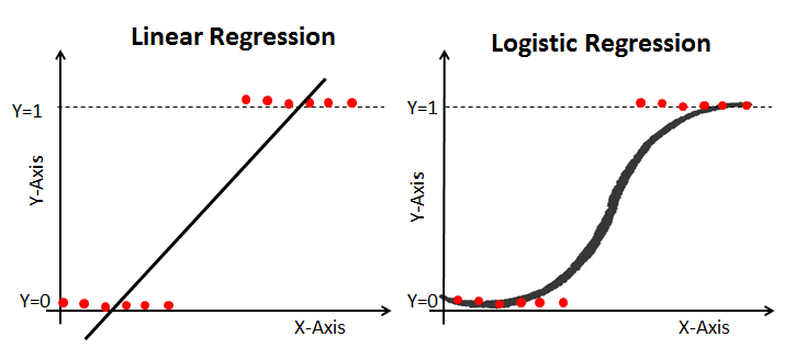
https://web.stanford.edu/~jurafsky/slp3/5.pdf

from sklearn.linear_model import LogisticRegression
import numpy as np
y = [0]*5 + [1]*5
X = np.array(list(range(10))).reshape(-1, 1)
print(X)
clf = LogisticRegression(random_state=0).fit(X, y)
print(clf.predict(X/1.6))

[[0]
 [1]
 [2]
 [3]
 [4]
 [5]
 [6]
 [7]
 [8]
 [9]]
[0 0 0 0 0 0 0 0 1 1]

6.13.8. Linear Regression Vs. Logistic Regression

Linear regression is frequently estimated using Ordinary Least Squares (OLS) while logistic regression is estimated using Maximum Likelihood Estimation (MLE) approach.

6.13.9. example1

https://youtu.be/g335THJxkto

берешь подмножество признаков - строишь линейную регрессию предсказывая какой-то другой признак - если ошибка стремится к нулю - есть зависимость

бывает что какие-то значения признаков хорошо группируют строки - решение средние значения таргета для разных групп

создаем новую переменную - среднее значение таргета для данной переменной

Подсчет статистик по таргету хорошо работает где есть категориальные признаки

6.13.10. example2

https://habr.com/ru/post/339250/

Скрытые зависимости между признаками могут описываться разными функциями, и в разных случаях разные функции могут проявить себя лучше остальных.
стоит изначально выбрать набор функций, адекватность применения которых зависит от специфики задачи.
Число производных столбцов для анализа равно k*(n² — n) / 2, где k — число выбранных функций F(Xi,Xj), n — число исходных признаков.
Для не очень большого числа признаков можно позволить себе полный перебор всех пар с полноценной проверкой полезности для каждого полученного признака.
Или быстрое отбрасывание самых неинформативных производных признаков и последующий более качественный разбор оставшихся.
Гипотетически есть возможность вычисления производных признаков F(Xi, Xj) от множества признаков M', которые даст нам применение метода главных компонент на исходное множество признаков M, но встаёт вопрос о том, все ли скрытые зависимости в этом случае могут быть проявлены.

6.13.11. links

6.14. Факторный анализ

Узучает variability одних переменных(видимых) с точки зрения других переменных(невидимых) меньшего количества.

Использует корреляционный анализ

6.15. Time Series Analysis

Univariate and Multivariate time series - y or (x,y,z).

6.15.1. terms

Structural break: unexpected change over time in the parameters of regression models, which can lead to huge forecasting errors

6.15.2. forecasting methods

Autoregression (AR)
Moving Average (MA)
Autoregressive Moving Average (ARMA)
Autoregressive Integrated Moving Average (ARIMA)
Seasonal Autoregressive Integrated Moving-Average (SARIMA)
Seasonal Autoregressive Integrated Moving-Average with Exogenous Regressors (SARIMAX)
Vector Autoregression (VAR)
Vector Autoregression Moving-Average (VARMA)
Vector Autoregression Moving-Average with Exogenous Regressors (VARMAX)
Simple Exponential Smoothing (SES)
Holt Winter’s Exponential Smoothing (HWES)

https://machinelearningmastery.com/time-series-forecasting-methods-in-python-cheat-sheet/

6.15.3. forecasting loss metrics

MAE Mean Absolute Error
RMSE - Root Mean Squared Error
MAPE - Mean Absolute Percentage Error
SMAPE - Symmetric Mean Absolute Percentage Error
коэффициент детерминации или R^2 = 1 - RSS/TSS'

Сравнение моделей прогнозирования с точки зрения баланса между точностью предсказания и сложностью (кол-вом параметров модели) применяется критерий Акаике (AIC)

AIC = 2 lnL + 2k
k = число параметров модели
L - соответствующее значение функции правдоподобия модели.

6.15.4. features

see 6.9.11.4

временные интервалы между измерениями постоянны или меняются?
тренд - плавное долгосрочное изменение уровня ряда
цикл - изменение уровня ряда с переменным перидом
шум - прогнозируемая случайная компонента ряда.
стационарность - ряд сгенерирован стационарным процессом

6.15.5. определение стационарности

автокорреляция ACF - является корреляцией сигнала с задержанной копией - или задержкой - самого себя как функция задержки.

коррелограмма), значения имеют тенденцию быстро уменьшаться до нуля для стационарных временных рядов

https://www.jstor.org/stable/3879300?seq=1#metadata_info_tab_contents

, [ Нильсен, 2006 ] предполагает, что построение коррелограмм на основе как автокорреляций, так и масштабированных автоковариаций и сравнение их обеспечивает лучший способ различения стационарных и нестационарных данных.

Параметрические испытания - статистические тесты, разработанные для обнаружения

Модульные корневые тесты

Тест Дики-Фуллера - в statsmodels а также ARCH пакеты.
Тест КПСС KPSS тест, [Kwiatkowski et al, 1992]

Тест Зивота и Эндрюса - допускает возможность структурный разрыв https://machinelearningmastery.ru/detecting-stationarity-in-time-series-data-d29e0a21e638/

6.15.6. rate of change

forward = (f(t2) - f(t1)) / △t
backward = (f(t1) - f(t2)) / △t
center = (f(t3) - f(t1)) / 2△t

np.diff - a[i+1] - a[i]

measurements = [2,3,4,4,3] # 5
dt = [1,1,2,3] # 4
import numpy as np
print( np.diff(measurements))
print( np.diff(measurements) / dt)
# print(list(reversed(measurements)))
# print("backward" np.diff(list(reversed(measurements))) / dt)
print( np.diff(measurements) / (np.array(dt)*2))

[ 1  1  0 -1]
[ 1.          1.          0.         -0.33333333]
[ 0.5         0.5         0.         -0.16666667]

https://e2eml.school/rate_of_change

6.15.7. one dimension convolution

Convolution vs. cross-correlation

https://en.wikipedia.org/wiki/Cross-correlation

autocorrelation - cross-correlate a signal with itself

https://e2eml.school/convolution_one_d

6.15.8. graphs

simple plot plt.plot - x - date, y - value
two sides simple plot
each year as a separate line in the same plot - Seasonal Plot of a Time Series
Boxplot of Month-wise (Seasonal) and Year-wise (trend) Distribution

two sides simple plot

fig, ax = plt.subplots(1, 1, figsize=(16,5), dpi= 120)
plt.fill_between(x, y1=y1, y2=-y1, alpha=0.5, linewidth=2, color='seagreen')
plt.ylim(-800, 800)
plt.title('Air Passengers (Two Side View)', fontsize=16)
plt.hlines(y=0, xmin=np.min(df.date), xmax=np.max(df.date), linewidth=.5)
plt.show()

TODO Boxplot of Month-wise (Seasonal) and Year-wise (trend) Distribution

6.15.9. datasets

Panel data df = pd.read_csv('https://raw.githubusercontent.com/selva86/datasets/master/MarketArrivals.csv')
Monthly anti-diabetic drug sales in Australia from 1992 to 2008. df = pd.read_csv('https://raw.githubusercontent.com/selva86/datasets/master/a10.csv', parse_dates=['date'], index_col='date')

6.15.10. TODO forecasting

https://facebook.github.io/prophet/

6.15.11. links

https://www.machinelearningplus.com/time-series/time-series-analysis-python/
Time Series Analysis, Regression, and Forecasting https://timeseriesreasoning.com/

6.16. Feature Importance

Нет однозначного ответа.

корреляция с таргетом
Random forest feature importance
NN - impotance путем перестановки значений поочереди в столбцах

Permutation feature importance - для любых моделей, путем перемешивании каждого столбца по очереди.

6.16.1. классификационные модели показывающие важность признаков

Random Forest, DesigionTreeClassification, DesigionTreeRegression
линейная модель с Lasso регуляризацией, склонной обнулять веса слабых признаков

p-values, bootstrap scores, various "discriminative indices"

Вычисление credible interval (частотный)

https://www.kaggle.com/shawlu/understanding-credible-interval

# 1 ----------------
import numpy as np
import scipy.stats

def mean_confidence_interval(data, confidence=0.95):
    a = 1.0 * np.array(data)
    n = len(a)
    m, se = np.mean(a), scipy.stats.sem(a)
    h = se * scipy.stats.t.ppf((1 + confidence) / 2., n-1)
    return m, m-h, m+h
# 2 ----------------
import numpy as np, scipy.stats as st
st.t.interval(0.95, len(a)-1, loc=np.mean(a), scale=st.sem(a))

# 3 ----------------
import statsmodels.stats.api as sms
sms.DescrStatsW(a).tconfint_mean()

# 4 ----------------
# Монетка

TODO Вычисление confidence interval (баесовый)

https://www.kaggle.com/shawlu/understanding-credible-interval

# 1 ----------------
import numpy as np
import scipy.stats

def mean_confidence_interval(data, confidence=0.95):
    a = 1.0 * np.array(data)
    n = len(a)
    m, se = np.mean(a), scipy.stats.sem(a)
    h = se * scipy.stats.t.ppf((1 + confidence) / 2., n-1)
    return m, m-h, m+h
# 2 ----------------
import numpy as np, scipy.stats as st
st.t.interval(0.95, len(a)-1, loc=np.mean(a), scale=st.sem(a))

# 3 ----------------
import statsmodels.stats.api as sms
sms.DescrStatsW(a).tconfint_mean()

# 4 ----------------

quantile loss method

6.19. Ensembles

https://scikit-learn.org/stable/modules/ensemble.html#voting-classifier
https://mlwave.com/kaggle-ensembling-guide/
https://en.wikipedia.org/wiki/Ensemble_learning
rus article https://dyakonov.org/2017/03/10/c%D1%82%D0%B5%D0%BA%D0%B8%D0%BD%D0%B3-stacking-%D0%B8-%D0%B1%D0%BB%D0%B5%D0%BD%D0%B4%D0%B8%D0%BD%D0%B3-blending/
Performance stop growing when I add more than 4 good models into the ensemble.
it helps to add some mediocre models

decrease the variance of a single estimate

Для регрессии ансамблирование происходит посредством уследнения результата каждой модели (Averaging)

метапризнаки - предсказания базовых моделей

метамодель - предиктор вход которого использует метапризнаки

6.19.1. stacking vs bagging vs boosting (old):

Бэггинг (баггинг, bagging, bootstrap aggregating): параллельное независимое построение моделей на различных наборах данных с последующим выбором предсказания по результатам голосования моделей(например мажоритарное голосование majority vote).
- Стекинг (stacking): построение k моделей базовых учеников (не обязательно одной природы) с дальнейшей подгонкой модели под метаклассификатор, обучение на одних и тех же данных
  - Смешивание (blending, блендинг): усреднение прогнозов группы моделей. multiple different algorithms are
  prepared on the training data. uses the held out validation set for that, typically 10% of instances are used for this purpose. Упрощенная модель стекинга.
Бустинг (boosting): последовательное построение моделей, при котором каждая модель учится с учетом результатов предыдущей модели. Чтобы избежать ошибок переобучения, каждая новая модель учится на результатах всех предыдущих моделей.
- AdaBoost

technique	pros	cons
bagging	parallel, lower variance	одинаковые модели, глубокие деревья
stacking	parallel	качество стльно зависит от базовых моделей
boosting	lower bias смещение	плохо параллелится
	модели уточняют друг-друга, простые базовые

6.19.2. stacking vs bagging vs boosting

Bagging: Simple voting or averaging of predictions.
- Bagged Decision Trees (canonical bagging)
- Random Forest
- Extra Trees
Stacking: 1. Different machine learning algorithms for each ensemble member. 2. Machine learning model to learn how to best combine predictions.
- Stacked Models (canonical stacking)
- Blending
- Super Ensemble
Boosting: 1. Bias training data toward those examples that are hard to predict. 2. Combine predictions using a weighted average of models.
- AdaBoost (canonical boosting)
- Boosting Machines
- Gradient Boosting (XGBoost and similar)

Bagging:
           +----------+
           | Input(X) |
           +----+++---+
              -/ | \-
            -/   |   \-
          -/     |     \-
        -/      /        \
      -/        |         \-
+----V---+ +----V---+ +-----V--+
| Sample1| | Sample2| | Sample3|
+----+---+ +----+---+ +----+---+
     |          |          |
+----V---+ +----V---+ +----V---+
| Tree1  | | Tree2  | | Tree3  |  --- model
+-----+--+ +----+---+ +--+-----+
       \--      |      -/
          \-    |   --/
            \-- | -/
               \+/
           +----V----+
           | Combine |            --- model
           +---------+
                |
           +----V----+
           | Output  |
           +---------+


Stacking:
           +----------+
           | Input(X) |
           +----+++---+
              -/ | \-
            -/   |   \-
          -/     |     \-
        -/      /        \
      -/        |         \-
+----V---+ +----V---+ +-----V--+
| Model1 | | Model2 | | Model3 |
+----+---+ +--------+ +--------+
       \--      |      -/
          \-    |   --/
            \-- | -/
               \+/
           +----V----+
           |  Model  |
           +---------+
                |
           +----V----+
           | Output  |
           +---------+

Boosting:

 +----------+
 | Input(X) |
 +----+-----+
      |
      +-------------+--------------+--------------+
      |             |              |              |
      |        +----v-----+        |              |
 +----v-----+  | Weighted |        |              |
 | Model1   +--> Sample1  |        |              |
 +----+-----+  +----+-----+        |              |
       \            |              |              |
       |            |         +----v-----+        |
        \      +----v-----+   | Weighted |        |
         \     | Model2   +---> Sample2  |        |
         |     +----+-----+   +----+-----+        |
          \         |              |         +----v-----+
           \        |         +----v-----+   | Weighted |
           |        |         | Model3   +---> Sample3  |
            \       |         +----+-----+   +----+-----+
             \      |            -/               |
             |      |          -/                 |
              \    /          /              +----v-----+
               \   |        -/               |   ...    |
               |   |      -/                 +--+-------+
                \  |     /             -------/
                 \ |   -/       ------/
                 | | -/ -------/
                  \|/--/
              +----v-----+
              | Combine  |
              +----+-----+
                   |
              +----v-----+
              |  Output  |
              +----------+

https://machinelearningmastery.com/tour-of-ensemble-learning-algorithms/

6.19.3. Stacking

Linear Stacking and Bayes optimal classifier or Stacked Generalization или Stacking - в задаче регрессии их среднее, а в задаче классификации — голосование по большинству, часто превосходят по качеству все эти алгоритмы.

stacking(5%) - X -> [Y] -> Y предсказывает основываясь на предсказаниях (предикторы)

тренируются алгоритмы
тренируется обобщающий алгоритм

Обучаем базовые модели на одних фолдах, проверяя на других мы уменьшаем риск переобучения

недостатки:

использование разных моделей требует подбирание гиперпараметров под каждый

Blending

6.19.4. bagging (bootstrap aggregation)

bagging trains each model in the ensemble using a randomly drawn subset of the training set.

The trick is that each sample of the training dataset is different, giving each classifier that is trained, a subtly different focus and perspective on the problem.

модели обучаются паралельно!

пример:

случайный лес

6.19.5. boosting

исходные данные модифицируются каждым алгоритмов в ансамбле

чаще выбираются входные данные показавшие ошибку
добавляются веса

недостатки

модели обучаются последовательно, поэтому используются слабые модели для скорости

пример:

градиентный бустинг над деревьями

6.19.6. skillfactory apporach

bootstarp + bagging
L1, L2, L3, L4 of random features
decision tree 1,2,3,4
мажоритарное голосование

6.20. Проверка гипотез

величину (значение) переменной называют статисти́чески зна́чимой, если мала вероятность ее случайного возникновения или ещё более крайних величин.

Null hypothesis (H0) - предположение о том, что не существует связи между двумя наблюдаемыми событиями, феноменами
- augmented Dickey–Fuller test (ADF)
Альтернатива (H1)

6.21. Автокорреляция ACF

Изучаются в:

анализ временных рядов
пространственная эконометрика

Автокорреляция - обычная корреляция Pearson между рядом и его версией сдвинутой на t+лаг

lag 0 - corr = +1
lag 1 - corr = 0.8
автокорреляция шума - слабо коррелированного процесса:
- имеет один пик lag 0
- при малейшем сдвиге corr сразу падает до нуля
uncorrelated does not necessarily mean random.

Выборочная автокорреляция -

Коррелограмма - диаграмма автокорреляционной функции

6.21.1. plotting

https://stackoverflow.com/questions/36038927/whats-the-difference-between-pandas-acf-and-statsmodel-acf

pandas.plotting.autocorrelation_plot(loan_amt.tail(1000)[::7]) - get every 7 record
statsmodels.graphics.tsaplots.plot_acf
matplotlib.pyplot.acorr(data.astype(float),maxlags=10) # -10, +10
- detrend: optional parameter. Default value: mlab.detrend_none.
- normed: True
- usevlines: Default value: True.
- maxlags: Default value: 10
- linestyle: optional parameter used to plot the data points when usevlines is False.
- marker: optional parameter having string value. Default value: ‘o’

6.21.2. calc

df['cost_requested'].autocorr() # lag=1 - Pearson correlation series and shifted self
np.corelate(a,v,mode=) modes:
- valid -
- same -
- full - от -len до +len

6.21.3. похожие понятия

взаимно-корреляционная функция
cross-correlation - measure of similarity of two series as a function of the displacement of one relative to the other
convolution - mathematical operation on two functions (f and g) that produces a third function (f*g) that expresses how the shape of one is modified by the other.
Partial Autocorrelation Function (PACF)
partial correlation measures the degree of association between two random variables, with the effect of a set of controlling random variables removed

6.21.4. – СРАВНЕНИЕ СПОСОБОВ – https://stackoverflow.com/questions/643699/how-can-i-use-numpy-correlate-to-do-autocorrelation

import numpy
import matplotlib.pyplot as plt

def autocorr1(x,lags):
    '''numpy.corrcoef, partial'''

    corr=[1. if l==0 else numpy.corrcoef(x[l:],x[:-l])[0][1] for l in lags]
    return numpy.array(corr)

def autocorr2(x,lags):
    '''manualy compute, non partial'''

    mean=numpy.mean(x)
    var=numpy.var(x)
    xp=x-mean
    corr=[1. if l==0 else numpy.sum(xp[l:]*xp[:-l])/len(x)/var for l in lags]

    return numpy.array(corr)

def autocorr3(x,lags):
    '''fft, pad 0s, non partial'''

    n=len(x)
    # pad 0s to 2n-1
    ext_size=2*n-1
    # nearest power of 2
    fsize=2**numpy.ceil(numpy.log2(ext_size)).astype('int')

    xp=x-numpy.mean(x)
    var=numpy.var(x)

    # do fft and ifft
    cf=numpy.fft.fft(xp,fsize)
    sf=cf.conjugate()*cf
    corr=numpy.fft.ifft(sf).real
    corr=corr/var/n

    return corr[:len(lags)]

def autocorr4(x,lags):
    '''fft, don't pad 0s, non partial'''
    mean=x.mean()
    var=numpy.var(x)
    xp=x-mean

    cf=numpy.fft.fft(xp)
    sf=cf.conjugate()*cf
    corr=numpy.fft.ifft(sf).real/var/len(x)

    return corr[:len(lags)]

def autocorr5(x,lags):
    '''numpy.correlate, non partial'''
    mean=x.mean()
    var=numpy.var(x)
    xp=x-mean
    corr=numpy.correlate(xp,xp,'full')[len(x)-1:]/var/len(x)

    return corr[:len(lags)]


if __name__=='__main__':

    y=[28,28,26,19,16,24,26,24,24,29,29,27,31,26,38,23,13,14,28,19,19,\
            17,22,2,4,5,7,8,14,14,23]
    y=numpy.array(y).astype('float')

    lags=range(15)
    fig,ax=plt.subplots()

    for funcii, labelii in zip([autocorr1, autocorr2, autocorr3, autocorr4,
        autocorr5], ['np.corrcoef, partial', 'manual, non-partial',
            'fft, pad 0s, non-partial', 'fft, no padding, non-partial',
            'np.correlate, non-partial']):

        cii=funcii(y,lags)
        print(labelii)
        print(cii)
        ax.plot(lags,cii,label=labelii)

    ax.set_xlabel('lag')
    ax.set_ylabel('correlation coefficient')
    ax.legend()
    plt.show()

6.22. Оптимизацинные задачи Mathematical Optimization Математическое программирование

6.22.1. definition

задача оптимизации сводится к нахождению экстремума целевой функции

The constraints of the problem can be used directly in producing the optimal solutions. There are algorithms that can solve any problem in this category, such as the popular simplex algorithm.

If a problem additionally requires that one or more of the unknowns must be an integer then it is classified in integer programming or integer linear programs.

A linear programming algorithm can solve such a problem if it can be proved that all restrictions for integer values are superficial, i.e., the solutions satisfy these restrictions anyway.

In the general case, a specialized algorithm or an algorithm that finds approximate solutions is used, depending on the difficulty of the problem.

решается:

эвристический алгоритм - heuristic (from Greek εὑρίσκω "I find, discover") is a technique designed for solving a problem more quickly when classic methods are too slow, or for finding an approximate solution when classic methods fail to find any exact solution
- Градиентный спуск gradient descent
- имитации отжига Simulated annealing [əˈnēl] -
- genetic algorithm - maintain a pool of solutions rather than just one. New candidate solutions are generated not only by "mutation" (as in SA), but also by "recombination" of two solutions from the pool.
- Simulated annealing [əˈnēl] - better than gradient descent, but more time consuming
- Quantum annealing - will usually give better results, it will have problems finding global minimum surrounded by large area of high values, because if it does not hit the small low area early, it won't get there after the parameter decreases.

6.22.2. terms

y - Критерием оптимальности, на основании его составляется целевая функция
целевая цункция objective function f(x) which output you are trying to min or max
variables x1,x2…
constaints - how big and small some variables may be
the feasible region defined by all values of x such that A x ≤ b and ∀ i , x i ≥ 0 is a (possibly unbounded) convex polytope.
basic feasible solution (BFS) - An extreme point or vertex of this polytope.

6.22.3. problem forms

problem - canonical form

Find a vector x that maximizes cT*x

subject to A*x <= b and x >= 0
problem - standard form
Linear function to be maximized:
- f(x1, x2) = c1*x1 + c2*x2
Problem constraints:
- a11*x1 + a12*x2 <= b1
- a21*x1 + a22*x2 <= b2
- a31*x1 + a32*x2 <= b3
Non-negative variables:
- x1 >= 0
- x2 >= 0
Problem:
- max{ cTx | x ∈ Rn ^ A*x<=b ^ x>=0 }
constrains inequalities to equalities and "standrad maximum form"
lets:
```
f = x1 + 2*x2
15*x1 + 10*x2 <= 1200
1*x1 + 2*x2 <= 120
x1, x2 >=0
```
```
15*x1 + 10*x2 <= 1200
```
difference bettween 15*x1 + 10*x2 and 1200 will be "slack variable" x3
```
15*x1 + 10*x2 + x3 = 1200
1*x1 + 2*x2 + x4 = 120
x1, x2 >=0  - not changed
-x1 - 2*x + f = 0
```
it is standrad maximum form:
- the objective fuction is to be maximized, so the leading coefficients are negative in the matrix
- the constraints are all <=, resulting in positive coefficients for slack variables
problem - tableau ['tæbləu] form (живая картина)
```
[ 1 -cT 0 ]
[ 0  A  b ]
```
for problem above in simplex tableu:
```
  x1 x2 x3 x4 f   ans
[ 15 10 1  0  0  1200 ]
[  1  2 0  1  0   120 ]
[ -1 -2 0  0  1     0 ]
```
basic variables: x3 and x4, objective fuction is f
linear constraint standard format
- x0 + 2*x1 <= 1
- 2*x0 + x1 = 1
```
-∞ <= 1 2 <= 1
1     2 1    1
```

6.22.4. TODO simplex algorithm

Z = -2*x - 3*y - 4*z minimize

subject to:

3*x + 2*y + z <= 10
2*x + 5*y + 3*z <= 15
x,y,z >= 0

canonical tableau:

[ 1 2 3 4 0 0 0  ]
[ 0 3 2 1 1 0 10 ]
[ 0 2 5 3 0 1 15 ]

slack variables s and t, column 5 and 6, basic feasible solution:

x = y = z = 0, s = 10, t = 15

Simplex method:

Convert a word problem into inequality constraints and an objective fuction.
Add slack variables, convert the objective function and build an initial tableau.
Choose a pivot.
Pivot
Repeat steps 3 and 4 until done.

6.22.5. good known problems

combinatorial optimization
In many such problems, such as the ones previously mentioned, exhaustive search is not tractable, and so specialized algorithms that quickly rule out large parts of the search space or approximation algorithms must be resorted to instead.
- exhaustive search is not tractable - исчерпывающий поиск невозможен
1. Knapsack problem ['næpsæk] рюкзак
  
  combinatorial optimization
  1. 0-1 knapsack problem
    Which restricts the number xi of copies of each kind of item to zero or one.
    - W - maximum weight capacity
    - n - items numbered from 1 up to n. each with weight wi and a value 𝞾i.
    maximize: (i=1..n)∑n𝞾i*xi
    
    subject to: ∑wi*xi <= W and xi ∈ Z, xi >= 0
    
    types:
    - weakly NP-complete - If the weights and profits are given as integers
    - strongly NP-complete - if the weights and profits are given as rational numbers.
2. Change-making problem
  
  finding the minimum number of coins (of certain denominations) that add up to a given amount of money.
  
  It is a special case of the integer knapsack problem.
3. Partition problem or number partitioning
  
  Special case of change-making problem.
  
  Deciding whether a given multiset S of positive integers can be partitioned into two subsets S1 and S2 such that the sum of the numbers in S1 equals the sum of the numbers in S2 (sum(S1) == sum(S2)).
  
  multiset - allows for multiple instances for each of its elements.
4. travelling salesman problem ("TSP")
5. minimum spanning tree problem ("MST")
Cutting stock problem
Packing problems

Bin packing problem: items of different sizes must be packed into a finite number of bins or containers, each of a fixed given capacity.

Subclass or form of Cutting stock problem.
Covering problems

ask whether a certain combinatorial structure 'covers' another, or how large the structure has to be to do that
Combinatorial auction (multi-lot auction)

special case of Smart market
TODO suffix trees
Generalized assignment problem
classic assignment problem

subclass of Generalized assignment problem
Weapon target assignment problem

finding an optimal assignment of a set of weapons of various types to a set of targets in order to maximize the total expected damage done to the opponent.

There are a number of weapons and a number of targets. The weapons Wi are of type i = 1 , … , m. Targets Vj are j = 1 , … , n. Any of the weapons can be assigned to any target. Each weapon type has a certain probability of destroying each target, given by p_ij.

Notice that as opposed to the classic assignment problem or the generalized assignment problem, more than one agent (i.e., weapon) can be assigned to each task (i.e., target) and not all targets are required to have weapons assigned.

6.22.6. Optimization with Calculus

TODO finding function zeroes(root, x-intercept or solution). Newton's method.
TODO guessing at the limiting slope. finding it with derivatives
TODO finding maximum and minimum values (without referencing or second derivatives)

6.22.7. имитация отжига

https://habr.com/ru/post/209610/

Нужно определить функции

E:S -> R S - состояния
T:N -> R N - номер итарации - убывающая функция изменения температуры
F:S -> S - порождающая новое состояние-кандидат

алгоритм

На входе: минимальная температура tmin, начальная температура tmax
Задаём произвольное первое состояние s1
Пока ti>tmin
1. S = F(s)
2. diff E = E(s) - E(s-1)
3. Если diff E<=0 , тогда состояние остается
4. Иначе переходим в новое состояние с вероятностью P(diff E, ti)
5. Понижаем температуру ti=T(i)
Возвращаем последнее состояние s

6.22.8. course

x_ij - сколько забирается со i склада клиенту j f = ∑{i,j} cost_{ij} * x_{ij}

Для каждого склада количество взятых предметов должно быть меньше, чем на складе:

\[\forall i: \sum_j x_{ij} \leq stock_i\]

Для каждого клиента количество приобретаемых товаров должно быть больше на единицу, чем спрос:

\[\forall j: \sum_i x_{ij} \geq demand_j\]

Который также:

\[\forall j: - \sum_i x_{ij} \leq -demand_j\]

from scipy.optimize import linprog
import numpy as np
cost = np.array([ # цены
    [2, 5, 3], # 1 склад - 1 2 3 клиент
    [7, 7, 6] # 2 склад - 1 2 3 клиент
])
stock = np.array([180,
                  220]) # наличие ресурсов на складе 1 и 2
demand = np.array([110, 150, 140]) # клиентам требуется ресурсов
num_warehouse = 2
num_clients = 3

A = []
b = []
for i in range(0, num_warehouse):
    A.append([0] * (num_clients * i) + [1] * num_clients + [0] * (num_clients * (num_warehouse - i - 1)))
    b.append(stock[i])
A = np.asarray(A)
b = np.asarray(b)
print(A)
print(b)

A = A.tolist()
b = b.tolist()
for j in range(0, num_clients):
    A.append(([0] * j + [-1] + [0] * (num_clients - j - 1)) * num_warehouse)
    b.append(-demand[j])
A = np.asarray(A)
b = np.asarray(b)

print("A", A)
print("b", b)
print("c", c)

print(linprog(c=c, A_ub=A, b_ub=b))

[[1 1 1 0 0 0]
 [0 0 0 1 1 1]]
[180 220]
A [[ 1  1  1  0  0  0]
 [ 0  0  0  1  1  1]
 [-1  0  0 -1  0  0]
 [ 0 -1  0  0 -1  0]
 [ 0  0 -1  0  0 -1]]
b [ 180  220 -110 -150 -140]
c [2 5 3 7 7 6]
        message: Optimization terminated successfully. (HiGHS Status 7: Optimal)
        success: True
         status: 0
            fun: 1900.0
              x: [ 1.100e+02  0.000e+00  7.000e+01  0.000e+00  1.500e+02
                   7.000e+01]
            nit: 5
          lower:  residual: [ 1.100e+02  0.000e+00  7.000e+01  0.000e+00
                              1.500e+02  7.000e+01]
                 marginals: [ 0.000e+00  1.000e+00  0.000e+00  2.000e+00
                              0.000e+00  0.000e+00]
          upper:  residual: [       inf        inf        inf        inf
                                    inf        inf]
                 marginals: [ 0.000e+00  0.000e+00  0.000e+00  0.000e+00
                              0.000e+00  0.000e+00]
          eqlin:  residual: []
                 marginals: []
        ineqlin:  residual: [ 0.000e+00  0.000e+00  0.000e+00  0.000e+00
                              0.000e+00]
                 marginals: [-3.000e+00 -0.000e+00 -5.000e+00 -7.000e+00
                             -6.000e+00]
 mip_node_count: 0
 mip_dual_bound: 0.0
        mip_gap: 0.0

```stdout [[1 1 1 0 0 0] [0 0 0 1 1 1]] [180 220]

Ответ: 110 единиц со склада 1 клиенту 1, 0 единиц со склада 1 клиенту 2, 70 единиц со склада 1 клиенту 3 0 единиц со склада 2 клиенту 1, 150 единиц со склада 2 клиенту 2, 70 единиц со склада 2 клиенту 3

6.22.9. scipy

Unconstrained minimization of multivariate scalar functions (minimize)
Objective functions in scipy.optimize expect a numpy array as their first parameter which is to be optimized and must return a float value.
- f(x, *args) where x represents a numpy array and args a tuple of additional arguments supplied to the objective function.
Constrained minimization of multivariate scalar functions (minimize)
Global optimization

finding global minima or maxima of a function (usually described as a minimization problem) (f = (-1) * g)
Least-squares minimization (least_squares)
Univariate function minimizers (minimize_scalar)
Custom minimizers
Root finding
Linear programming (linprog)
Assignment problems

6.22.10. links

https://web.stanford.edu/group/sisl/k12/optimization/#!index.md

6.23. Optimization algorithms

Optimization algorithms tend to be iterative procedures. Generate trial solutions that converge to a “solution”.

Deterministic Algorithm
Randomized Algorithm

types by complexity and speed:

Finite versus infinite convergence. For some classes of optimization problems there are algorithms that obtain an exact solution—or detect the unboundedness–in a finite number of iterations
Polynomial-time versus exponential-time. The solution time grows, in the worst-case, as a function of problem sizes (number of variables, constraints, accuracy, etc.)
Convergence order and rate: arithmetically, geometrically or linearly, quadratically.

Algorithm Classes depending on information of the problem being used to create a new iterate:

Zero-order: when the gradient and Hessian information are difficult to obtain, e.g., no explicit function forms are given, functions are not differentiable, etc.
First-order: large scale data optimization with low accuracy requirement. good for Machine Learning, Statistical Predictions.
Second-order: Popular for optimization problems with high accuracy need, e.g., some

scientific computing, etc.

https://web.stanford.edu/class/msande311/lecture09.pdf

6.24. виды графиков

Line chart [ʧɑːt]
- Scree plot (skriː) [plɒt] - Улучшенная Дендрограмма для иерархической кластирезации
- graph of a function
Scatter plot [ˈskætə] Диаграмма рассеяния - для демонстрации наличия или отсутствия корреляции между двумя переменными.
- 2D Histogram - температура скопления
pie chart - кусочки
bar plot or chart - Столбчатая диаграмма
гистограмма x-зачения y - количество таких значений
- по группам - данные разбиваются на группы и для каждой рисуется гистограмма
- kdeplot - проксимация линией
Box plot, Ящиковая диаграмма, Ящики с усами - свеча от quantile 1 - quantile 3, median = quantile 2. Толщина не имеет значения.
Q–Q plot or Probability plot - comparing two probability distributions - plotting their quantiles against each other or agains normal distribution.
AUC ROC Curve
Временные:
- ACF - x - лаг, y - корреляция
- PACF statsmodels
Correlation Matrix with Heatmap
Scatter matrix
Partial Dependence Plots PDP - shows the marginal effect one or two features have on the predicted outcome of a machine learning model
individual conditional expectation (ICE) plot - like PDP but visualizes the dependence of the prediction on a feature for each sample separately with one line per sample

6.24.1. простые линейные графики с описанием

from matplotlib import pyplot as plt plt.plot(list(n_m), gmm_model_comparision['AIC'], label='AIC') plt.plot(list(n_m), gmm_model_comparision['BIC'], label='BIC') plt.legend() plt.gca().set(xlabel='число кластеров', ylabel='оценка модели') plt.show()

6.24.2. форматирование axis

from matplotlib.ticker import FuncFormatter

def millions(x, pos):
    return '%1.1fM' % (x * 1e-6) # remove 6 digits

formatter = FuncFormatter(millions)
a = df.groupby('education')['cost_requested'].plot.hist()
a[0].xaxis.set_major_formatter(formatter)

6.24.3. гистограмма

df.groupby('education')['cost_requested'].plot.hist()
plt.legend()
plt.show()

6.24.4. box plot

boxplot = df.boxplot(column=['Col1', 'Col2', 'Col3'])

6.24.5. bar plot, bar chart

# Bar Chart Vertical
dfg = df.groupby('address_actual')['cost_requested'].agg('sum')
x = range(len(dfg))
plt.bar(x, dfg)
x_labels = df['address_actual'].unique()
plt.xticks(x, sorted(x_labels))
plt.xticks(rotation=60) # much better
plt.show()
# Horizontal Bar Chart
x = range(3)
plt.barh(x,[1,2,3])
plt.yticks(x, ['a','b','c'])
plt.show()

# Horizontal Bar Chart with center
import matplotlib
from pylab import *

val = 3-6*rand(5)    # the bar lengths        # changed your data slightly
pos = arange(5)+.5    # the bar centers on the y axis
print pos
figure(1)
barh(pos,val, align='center',height=0.1)    # notice the 'height' argument
yticks(pos, ('Tom', 'Dick', 'Harry', 'Slim', 'Jim'))

gca().axvline(0,color='k',lw=3)   # poor man's zero level

xlabel('Performance')
title('horizontal bar chart using matplotlib')
grid(True)
show()

6.24.6. Q–Q plot

import pylab  # Plotting
import scipy.stats as stats  # scintific calculation
stats.probplot(df['cost_requested'], dist="norm", plot=pylab)
pylab.show()

6.24.7. Scatter plot

# for two
x = df['cost_requested']
y = df['income']
plt.scatter(x, y)
plt.title('Диаграмма рассеяния')
plt.xlabel('cost_requested')
plt.ylabel('income')
plt.show()

# for three
plt.plot(x,y, 'b*', z, 'g^') # y -blue, z -green
plt.show()

6.24.8. Scatter matrix

по диаганали ядерные оценки плотности или сглаженные гистограммы

from pandas.plotting import scatter_matrix
colours = {0:'red', 1:'green'}
scatter_matrix(df[cols],
               diagonal='kde',
               c =df['result'].replace(colours))
plt.show()

6.24.9. Correlation Matrix with heatmap

cols = ['cost_requested', 'income', 'loan', 'charge']
corr = df[cols].corr()
plt.matshow(corr,  cmap=plt.cm.Reds)
# or
# plt.imshow(corr, cmap='RdYlGn', interpolation='none', aspect='auto')
tick_marks = [i for i in range(len(cols))]
plt.xticks(tick_marks, cols, rotation='vertical')
plt.yticks(tick_marks, cols)
plt.colorbar()
plt.title("Матрица корреляции")
plt.show()

6.24.10. PDP

https://scikit-learn.org/stable/modules/partial_dependence.html#partial-dependence

Влияние анкетного скоринга на решение модели

from sklearn.inspection import partial_dependence
from sklearn.inspection import plot_partial_dependence
from xgboost import XGBClassifier

X = df0.drop(['system'], 1)
X = X.drop(['under'], 1)
Y = df0[['system', 'under']]

# print(X.columns.values)
# exit(0)
# train model
model = XGBClassifier(booster='gbtree', objective='binary:logistic', scale_pos_weight=45, max_depth=3,
                      learning_rate=0.1, gamma=1, num_round=4)
est = model.fit(X, Y['under'])

# a = partial_dependence(est, features=[0], X=X, percentiles=(0, 1), grid_resolution=2)
# print(a)
X_uses = X[X['`condition`_uses'] == 1]
_ = plot_partial_dependence(est, X_uses, features=['anket_score'], n_jobs=4, grid_resolution=20)

6.24.11. pie chart

Распределение чего-то между чем-то. Когда 100 процентов делится между кем-то

6.24.12. sns.lmplot для 2 столбцов (scatter + regression)

sns.lmplot(data = df, x = 'Age', y = 'SprintSpeed',lowess=True,scatter_kws={'alpha':0.01, 's':5,'color':'green'}, line_kws={'color':'red'})

6.25. виды графиков по назначению

https://python-graph-gallery.com/ https://foxhugh.com/visual-communication/visualization-2/list-of-visualization-methods-3/

DISTRIBUTION
- VIOLIN
- DENSITY
- BOXPLOT
- HISTOGRAM
CORRELATION
- Scatterplot
- Connected Scatter plot
- Bubble plot
- Heatmap
- 2D density plot
- Correlogram
RANKING
- Barplot
- Boxplot
- parallel plot
- Lollipop plot
- Wordcloud
- Radar chart or Spider plot or Polar chart or Web chart
PART OF A WHOLE
- Stacked barplot
- Tree plot
- Venn diagram
- Doughnut plot
- Pie plot
- Tree diagram
EVOLUTION
- Line plot
- Area plot
- Stacked area plot
- Parrallel plot
- Streamchart
MAPS
- Map
- Choropleth map
- Connection map
- Bubble map
FLOW
- Chord diagram
- Network chart
- Sankey diagram
Other
- Animation
- Cheat sheet
- Data Art
- Color
- 3D
- Bad chart

6.26. библиотеки для графиков

Matplotlib
Plotly
Seaborn
Altair
Bokeh

6.27. тексты

Convert a collection of text documents to a matrix of token counts

from sklearn.feature_extraction.text import CountVectorizer

TF-IDF - оценка важности слова. Вес слова равен частоте употреблений в документе и обратно пропорционален частоте употреблений во всех докумнетах коллекции.

from sklearn.feature_extraction.text import TfidfTransformer

6.28. типичное значение

mean - среднее арифметическое 1+2+3/3
- если есть выброс - среднее будет больше 75 квантили или меньше 25
медиана - список сортируется и берется значение из середины 50/50, равна квартили 50%
усеченная средняя

6.29. simularity measure - Коэффициент сходства

безразмерный показатель сходства сравниваемых объектов.

унарные - меры разнообразия Diversity index и меры концентрации degree of concentration
- Diversity index - quantify the entropy
бинарные -
n-арные, многоместные

other terms:

Матрица мер конвергенции - similarity matrix ( recommender systems)
Contingency table - multivariate frequency distribution of the variables
- measure significance of the difference between the two proportions: Pearson's chi-squared test, the
G-test, Fisher's exact test, Boschloo's test, and Barnard's test.

Binary:

between sets, areas in object detection (CV):
- Jaccard index J(A,B) = |A⋃B| / |A⋂B| = |A⋂B| / (|A| + |B| - |A⋂B| ) - intersection of two sets / union of two sets
  - good for binary data
  - 0 <= J(A,B) <= 1
  - good for binary comparision = TP
  - Kj = c / a + b - c, where c is intersection of a and b
- Sorensen similarity index - the weight for the number of shared items is larger
- Sørensen–Dice coefficient (F1 score) 2*|A⋃B| / |A⋂B| = 1 - 2* |A⋂B| / (|A| + |B|)
between two data points: see 6.12.6.4
- Euclidean distance
- Manhattan distance
between vectors:
- Cosine simularity = ∑(Ai*Bi) / sqrt(∑Ai^2 * ∑Bi^2))
  - V and a*V are maximally similar.
  - Ko = c / sqrt(a*b)
  - good for embeddings, because embeddings is vectors and vectors close when sources is close.
  - not invariant to adding a constant to all elements
between strings
- Levenshtein distance

Cosine simularity = (| A - B | ^2) / 2 where |A|^2 = |B|^2

Correlation - linearly related x1*a+b = x2*c+d or x1*a1+x2*a2 + c = 0

partial correlation - measures the degree of association between two random variables, with the effect of a set of controlling random variables removed.
Pearson product-moment correlation
Rank correlation: Kendall's, Spearman's ρ (for ordinal data: like 1, neutral 2, dislike 3

Pearson vs cosine simularity.

Pearson invariant to adding any constant to all elements.
Pearson Correlation Coefficient and Cosine Similarity are equivalent when X and Y have means of 0.
Corr(x,y) = CosSim(x - mean(x), y - mean(x))

6.30. libs

ArviZ: Exploratory analysis of Bayesian models
statsmodels - provides classes and functions for the estimation of many different statistical models, as well as for conducting statistical tests, and statistical data exploration.
seaborn: statistical data visualization

6.31. decision tree

pros

easy to interpret
Can handle data of different types, including continuous, categorical, ordinal, and binary. Transformations of the data are not required.
Handle missing data by identifying surrogate splits in the modeling process. Surrogate splits are splits highly associated with the primary split. In other models, records with missing values are omitted by default.

cons

unstable
overfit

https://webfocusinfocenter.informationbuilders.com/wfappent/TLs/TL_rstat/source/DecisionTree47.htm

comparision of algorithms https://journals.plos.org/plosone/article?id=10.1371/journal.pone.0210236

Which is better Linear or tree-based models?

If you need to build a model that is easy to explain to people, a decision tree model will always do better than a linear model.

6.31.1. how it works

features are always randomly permuted at each split,

splits the nodes on all available variables and then selects the split which results in most homogeneous sub-nodes.
- function to measure the quality of a split: default=”squared_error”
- Different algorithms use different metrics for measuring "best": 1. calculates Entropy(H) and Information
gain(IG) of this attribute. 2. selects the attribute which has the smallest Entropy or Largest Information gain.
algorithm continues to recur on each subset, considering only attributes never selected before.

6.32. продуктовая аналитика

Продуктовый аналитик — это человек, который умеет:

оценить, какие действия и параметры пользователей в продукте нужно отслеживать;
настроить сбор этих данных;
создавать отчеты, графики для принятия продуктовых решений на основе собранных ранее данных.

Продуктовая аналитика помогает понять:

какие элементы продукта пользователи используют, а какие игнорируют;
какие сценарии внутри продукта приводят к покупке, а какие к отказам;
какие характеристики тех пользователей, кто становится клиентом, и тех кто уходит с продукта;
как меняется поведение пользователей в результате обновлений продукта.

встречу по уточнению бэклога (PBR-Product Backlog Refinement)

продуктовый аналитик – представитель владельца продукта на встрече с командой,

практику «3 амиго»,задачу с трех точек зрения:

контекст бизнес-задачи (что нужно бизнес-заказчику)
технический контекст (как это сделать)
контекст валидации решения (как мы узнаем, что сделали то, что нужно).

Продумывать дизайн A/B-тестов и интерпретировать их результаты; Добавлять новые метрики в систему A/B-тестов, проверять метрики на статистическую корректность; Развивать дашборды, позволяющие отвечать на вопросы о том, что происходит с продуктом; Проводить adhoc анализ данных о поведении пользователей.

Имеет опыт проведения A/B-тестов и теоретическую базу для их проведения: знает математическую статистику и теорию вероятностей; Имеет опыт создания дашбордов в Tableau или другой BI системе. Интересуется современными практиками визуализации данных;

6.33. links

https://www.kdnuggets.com/

7. Information retrieval

7.1. measures

Evaluation measures for IR - how well an index, search engine or database returns results from a collection of resources that satisfy a user's query

8. Recommender system

subclass of information filtering system

8.1. basic

ways:

Content-based filtering (or personality-based approach) - compare pre-tagged characteristics of an item with user profile.
- best suited when there is known data on an item, but not on the user.
collaborative filtering technique - user's past behavior
- requires a large amount of information about a user
- cold start problem is common in collaborative filtering systems
- memory-based and model-based
- advantage - does not rely on machine analyzable content and doesn't need to "understand" of the item itself.

types

Multi-criteria recommender systems
Risk-aware recommender systems
Mobile recommender systems
Hybrid recommender systems
knowledge-based systems
opinion-based recommender systems
Session-based recommender systems - mainly based on generative sequential models such as Recurrent Neural Networks, Transformers, and other deep learning based approaches.

recommender systems

Collaborative filtering (CF) - user's past behavior + similar decisions made by other users
- Model-based
  - clustering
Content-based
Hybrid models (CF + Content-based)

8.2. algorithms all

collaborative

user-based algorithm - memory-based
Matrix factorization (recommender systems) - model-based approaches
k-nearest neighbor (k-NN)
the Pearson Correlation as first implemented by Allen.
item-to-item collaborative filtering (people who buy x also buy y), an algorithm popularized by Amazon.com's recommender system

content based:

create user profile as a weighted vector of item features. The weights denote the importance of each feature.
Bayesian Classifiers
cluster analysis
decision trees
artificial neural networks in order to estimate the probability that the user is going to like the item.

hybridization techniques:

Weighted: Combining the score of different recommendation components numerically.
Switching: Choosing among recommendation components and applying the selected one.
Mixed: Recommendations from different recommenders are presented together to give the recommendation.
Feature Combination: Features derived from different knowledge sources are combined together and given to a single recommendation algorithm.[54]
Feature Augmentation: Computing a feature or set of features, which is then part of the input to the next technique.[54]
Cascade: Recommenders are given strict priority, with the lower priority ones breaking ties in the scoring of the higher ones.
Meta-level: One recommendation technique is applied and produces some sort of model, which is then the input used by the next technique.[55]

techs

Reinforcement learning
Multi-criteria recommender systems (MCRS) - multiple criteria of item that affect this overall preference value.
Risk-aware recommender systems - risk of disturbing the user with unwanted notifications - content-based technique and a contextual bandit algorithm.

fast:

Near-neighbor search in high dimensions (LSH). Take an item to quickly find a set of neighbors. This can be done once every day or every few hours.
clustering to search only within clusters.

8.3. matrix factorization

factor rating matrix "all users by all items" to multiplication of matrixes “all items by some taste dimensions” and “all users by some taste dimensions”. These dimensions are called latent or hidden features and we learn them from our data.

express each user as a vector of their taste values, and at the same time express each item as a vector of what tastes they represent

ways to factor a matrix:

Singular Value Decomposition (SVD)
Probabilistic Latent Semantic Analysis (PLSA)

For explicit data we treat missing data as just unknown fields that we should assign some predicted rating to. But for implicit we can’t just assume the same since there is information in these unknown values as well

ALS is an iterative optimization process where we for every iteration try to arrive closer and closer to a factorized representation of our original data.

R = U * V

V - vector for each item
U - vector for each user

simularity items score = V*VT

making recommendations score = Ui*VT, matrix transpose.

8.3.1. links

Collaborative filtering for Implicit Feedback Datasets http://yifanhu.net/PUB/cf.pdf
https://medium.com/radon-dev/als-implicit-collaborative-filtering-5ed653ba39fe

8.4. algoriths

8.4.1. memory based

ratings user u gives to item i is calculated as an aggregation of some similar users' rating of the item:

r_ui = aggr(r_u'i)

where u' is the set of N top users that most similar to user u, who rated item i.

aggr - may vary

disadvantages:

performance decreases when data gets sparse,
This hinders the scalability of this approach and creates problems with large datasets
Adding new items requires inclusion of the new item and the re-insertion of all the elements in the structure.

8.4.2. Model-based

dimensionality reduction methods are mostly being used as complementary technique to improve robustness and accuracy of memory-based approach, models often called "latent factor models". they compress user-item matrix into a low-dimensional representation in terms of latent factors.

models:

Bayesian networks, clustering models, latent semantic models such as singular value decomposition, probabilistic latent semantic analysis, multiple multiplicative factor, latent Dirichlet allocation and Markov decision process based models

low-dimensional representation utilied by user-based or item-based neighborhood algorithms see 8.4.1

8.4.3. Deep learning

Autoencoders
WIde and deep learning - linear algorithm + deep componen of emvedding vectors as a liner combination of output and trained together
Neural Graph Matching-Based CF (GMCF) - on graph neural network (GNN)

8.4.4. keras

https://keras.io/examples/structured_data/collaborative_filtering_movielens/ https://www.kaggle.com/code/faressayah/collaborative-filtering-for-movie-recommendations

Map user ID to a "user vector" via an embedding matrix
Map movie ID to a "movie vector" via an embedding matrix
Compute the dot product between the user vector and movie vector, to obtain the a match score between the user and the movie (predicted rating).
Train the embeddings via gradient descent using all known user-movie pairs.

8.4.5. pyTorch - TorchRec

platform https://github.com/pytorch/torchrec
Deep Learning Recommendation Model (DLRM)https://arxiv.org/abs/1906.00091
example (main in 502 line) https://github.com/facebookresearch/dlrm/blob/main/torchrec_dlrm/dlrm_main.py
- Criteo Terabyte Dataset https://labs.criteo.com/2013/12/download-terabyte-click-logs/
article(800 GPU) https://www.adityaagrawal.net/blog/dnn/dlrm
article https://medium.com/swlh/deep-learning-recommendation-models-dlrm-a-deep-dive-f38a95f47c2c
article (multi GPU) https://catalog.ngc.nvidia.com/orgs/nvidia/resources/dlrm_for_pytorch

8.4.6. TensorFlow Recommenders

8.4.7. Neural Graph Matching based Collaborative Filtering (GMCF)

https://github.com/ruizhang-ai/GMCF_Neural_Graph_Matching_based_Collaborative_Filtering https://arxiv.org/abs/2105.04067

8.4.8. DLRM vs GMCF

Both models are highly scalable DLRM 2019

ability to handle massive amounts of feature data
excels at capturing complex user-item relationships

GMCF 2021 pytorch

useful when there is limited user-item interaction data available
more adept at handling sparse and incomplete data
capture graph structure of user-item interactions

8.4.9. surprise

https://pypi.org/project/scikit-surprise/

8.5. datasets

MovieLens dataset https://grouplens.org/datasets/movielens/

ratings

userId
movieId
rating
timestamp

8.6. simularity

jaccard simularity - ignore rating values
centered cosine simularity - treats the unknown values as zeros. If we normalize by substractin mean - blank fields will be neutral.

items to items outperforms user to user, items simpler.

8.7. terms

cold start - the issue that the system cannot draw any inferences for users or items about which it has not yet gathered sufficient information
- New community
- New item
- New user
explicit and implicit forms of data collection. - explicit asking and implicit observing.
meta-data of items
user-item (utility) matrix or Rating Matrix

8.8. problems

Cold start
Scalability
Sparsity - most active users will only have rated a small subset of the overall database, most popular items have very few ratings
the value from the recommendation system is significantly less than when other content types from other services can be recommended - more for content based systems

8.9. scikit-surprise

https://rubikscode.net/2020/04/27/collaborative-filtering-with-machine-learning-and-python/ https://pypi.org/project/scikit-surprise/

8.10. links

8.10.1. Alternating Least Squares (ALS)

links

https://medium.com/radon-dev/als-implicit-collaborative-filtering-5ed653ba39fe

9. Machine learning

национальная тех инициатива, хуйня какае-то http://www.nti2035.ru/
офигенный блог End-to-End Machine Learning https://brohrer.github.io/blog.html
https://samoa.incubator.apache.org/
tadviser.ru http://www.tadviser.ru/index.php/%D0%A1%D1%82%D0%B0%D1%82%D1%8C%D1%8F:%D0%98%D1%81%D0%BA%D1%83%D1%81%D1%81%D1%82%D0%B2%D0%B5%D0%BD%D0%BD%D1%8B%D0%B9_%D0%B8%D0%BD%D1%82%D0%B5%D0%BB%D0%BB%D0%B5%D0%BA%D1%82_%D0%B2_%D0%B1%D0%B0%D0%BD%D0%BA%D0%B0%D1%85
scholar.google.ru - поисковая система по текстам научных публикаций
канал по статистике и машинное обучение https://www.youtube.com/channel/UCtYLUTtgS3k1Fg4y5tAhLbw
Cheatsheets https://ml-cheatsheet.readthedocs.io
2) Машинное обучение, чему учатся дебилы яндекса https://yandexdataschool.ru/edu-process/program/ml-dev
1) лекции по машинному обучению на русском http://www.machinelearning.ru/wiki/index.php?title=%D0%9C%D0%B0%D1%88%D0%B8%D0%BD%D0%BD%D0%BE%D0%B5_%D0%BE%D0%B1%D1%83%D1%87%D0%B5%D0%BD%D0%B8%D0%B5_%28%D0%BA%D1%83%D1%80%D1%81_%D0%BB%D0%B5%D0%BA%D1%86%D0%B8%D0%B9%2C_%D0%9A.%D0%92.%D0%92%D0%BE%D1%80%D0%BE%D0%BD%D1%86%D0%BE%D0%B2%29
3) http://sberbank.ai/
4) Google Deep Learning course https://www.udacity.com/course/deep-learning--ud730
главный сайт дата майнеров https://www.kdnuggets.com/
еще дата майнеры https://www.datasciencecentral.com
UCI ML Repository (349 datasets) https://archive.ics.uci.edu/ml
Яндекс Академия канал https://www.youtube.com/channel/UCKFojzto0n4Ab3CRQRZ2zYA/videos
блог сбера https://habr.com/en/company/sberbank/
Введение в архитектуры нейронных сетей 2017 https://habr.com/ru/company/oleg-bunin/blog/340184/
AI Journey 20.12.03 https://www.youtube.com/watch?v=mYvHDaQCRXc&list=PLdtmzrRhJMFITdlt-MYV2Wq6I_W-Ki0ZW&index=1

прикладной статистики, численных методов оптимизации, дискретного анализа -> интеллектуального анализа данных (data mining)

9.1. steps

ISO/IEC-23053 › Framework for Artificial Intelligence (AI) Systems Using Machine Learning (ML)

yandex ml course

бизнес задачи:

дашборды для метрик
бизнес запрос в задачу МЛ
готовит презентацию задачи заказчику

исследование

подбирает метод и силу регуляризации
исключает выбросы и ложные данные

инженерные

отбирает информативные признаки
разрабатывает пайплайн обучения модели
создает микросервис предсказаний
создает пайплайн трансформации данных

9.2. ensembles theory

9.2.1. terms

base learners: most ensemble methods use a single base learning algorithm to produce homogeneous base learners.
classification hyperplate: the boundary that separates the different classes in a classification problem.
merging or fusion: 1) distance from x in f(x) to the classification hyperplate 2) the process of combining the predictions or outputs generated by multiple individual models, in order to make a final prediction or decision 3) margin refers to the distance between the hyperplane and the closest data points from each class. A larger margin indicates a better separation between the classes.

9.2.2. history

Epicurus (341-270 B.C.): principle of multiple explanations - are consistent with empirical observations.

areas

combining classifiers - strong classifiers (recognition community)
ensembles of weak learners - (ml community)
mixture of experts - divide-and-conqure strategy (nn community)

1990 Hansen and Salamon: it was found that predictions made by the combination of a set of classifiers are often more accurate than predictions made by the best single classifier.

combination is nice
best single is good
average is the best

1990 Schapire: weak learners can be boosted to strong learners

9.2.3. b

Вопрос поднятый Michael Kearns and Вэлиант Лусли "Может ли набор слабых обучающих алгоритмов создать сильный обучающий алгоритм?"

утвредительный ответ http://www.cs.princeton.edu/~schapire/papers/strengthofweak.pdf

how base learners are generated:

sequential ensemble methods (with adaboost for ex) - exploit the dependence between the base learners. overall performace can be boosted in a residual-decreasing way.
parallel ensemble methods - exploit the independence between the base learners.

steps

Generating the base learners - accurate as possible and diverse as possible.
combining them.

with a large ensemble, there are a lot of weights to learn, and this can easily lead to overfitting

9.2.4. AdaBoost

reduces the error exponentially fast
in order to achieve a good generalization, it is necessary to constrain the complexity of base learners and number of learning rounds
often does not overfit - empirical.

9.2.5. Hoeffding's inequality

provides an upper bound on the probability that the sum of bounded independent random variables.

the sum of bounded independent random variables deviates from its expected value by more than a certain amount.

S = X1+ … + Xn, where Xn - independent random variables

9.2.6. TODO Bias-Variance Decompostion, Statistical Computational and Representational, Diversity

9.2.7. error rate

binary classification {-1, +1}, classificator hi, ground-truth function f:

independent generalization error: P(hi(x) != f(x)) = e

9.2.8. fusion strategy or combination methods

majority voting (hard voting) - 1) calc argmax per individual learner 2) select mode from all learners
Majority Voting
Bayes Optimal Classifier
Stacked Generalization
Super Learner
Consensus
Query-By-Committe

Weighted Average Probabilities (Soft Voting) - returns the class label as argmax of the sum of predicted
probabilities.
- steps: 1) calc average per class, 2) select max NN
- H(x) = sum(wi*hi(x)), i =1..T, wi>=0, sum(wi) = 1
- other combination methods are special cases of weighted averaging (Perrone and Cooper 1993)
- there is no evidence that weighted average is better than simple averaging
- good for combining learers with nonidentical strength
Averaging or Unweighted Model Averaging
- simple averaging: (1/T)*sum(hi(x))
  - err(H) <= err(h)
  - able to get err(H) = (1/T)*err(h), where T - count of learners, H - f of all.
  - does not have to learn any weights (less parameters) , and so suffer little from overfitting
  - good for combining learners with similar performance
Voting
- hi, i..T - classifiers
- cj, j..l - classes
majority voting - if more that half of classifiers votes for same class, else rejection option used.

9.2.9. links

https://github.com/PacktPublishing/Hands-On-Ensemble-Learning-with-Python
Ensemble Methods: Foundations and Algorithms - Zhi-Hua Zhou - 2012
2022 [2104.02395] Ensemble deep learning: A review https://arxiv.org/abs/2104.02395
https://scikit-learn.org/stable/modules/ensemble.html

9.3. Эвристика Heuristics

Эвристические техники - приблизительные техники основанные на прошлом опыте.
Эвристика - heuristic (hjʊəˈrɪstɪk) - ментальный багаж накопленных навыков.
Эвристика - то, что отличает человека от AI - совокупность приёмов и методов, облегчающих и упрощающих решение

познавательных, конструктивных, практических задач. Машинные эвристики в полтора раза хуже чем машиннео обучение Извесные:

Similarity heuristic - сравнение нового со старым чтобы сделать решение - learning from past
Take-the-best heuristic or Satisficing(threashold)
Fast-and-frugal trees
Fluency heuristic - if one object is processed more fluently, faster, or more smoothly than another, the mind infers that this object has the higher value with respect to the question being considered
Gaze heuristic - эвристика взгляда - как у охотника
recognition heuristic - If one of two objects is recognized and the other is not, then infer that the recognized object has the higher value with respect to the criterion.

Гештальт - целостная структура, отличная от суммы его частей

характерная тенденция психики к организации опыта в доступное пониманию целое
Целое может быть важным, члены — неважными, и наоборот. Фигура всегда важнее основы — фона.
Эффект Зейгарник - человек лучше запоминает прерванные действия, чем завершённые
примеров, по Кёлеру, является мелодия, которая узнаётся даже в случае, если она транспонируется в другие тональности.

Availability heuristic - reason why advertising exist.

9.3.1. links

9.4. Энтропия

непредсказуемость появления какого-либо символа первичного алфавита.

Двоичная энтропия для независимых случайных событий x или состояний системы:

H(x) = - (от i = 1 до n)∑pi*log2(pi) , где pi - вероятность x (i=1…n)
Частная энтропия Hi = -log2pi

9.5. Artificial general intelligence AGI or strong AI or full AI

Approaches:

9.5.1. Symbolic AI or Good Old Fashioned AI (GOFAI)

https://arxiv.org/pdf/1703.04368.pdf

based on high-level "symbolic" (human-readable) representations of problems, logic and search

"physical symbol systems hypothesis" - thinking is manipulation of symbols

symbols or strings are stored manually or incrementally in a Knowledge Base.
used to make intelligent conclusions and decisions based on the memorized facts and rules put together by propositional logic (Логика высказываний) or first-order predicate calculus techniques (First-order logic)

cons:

Patterns are not naturally inferred or picked up but have to be explicitly put together and spoon-fed to the system
dynamically changing facts and rules are very hard to handle
learning procedures are monotonically incremental

9.5.2. Others

Deep learning
Bayesian networks
Evolutionary algorithms

9.6. Machine learning

Randomized algorithms fall into two rough categories:

Las Vegas algorithms always return precisely the correct answer. Consume a random amount

of resources, usually memory or time. Use sampling. Approximate the expectation by a corresponding average.

Monte Carlo algorithms return answers with a random amount of error. Error can typically be reduced by expending more resources

MultiOutputClassifier(RandomForestClassifier(n_estimators = 100, n_jobs = 6))) - классификатор multi-target classification

9.6.1. ML techniques

linear

PCA

уменьшает размерность и возвращает новые "components" на которые проецируются все фичи

components_ - Principal Components - новые фичи на которые проецируются старые

How many principal components we can choose for our new feature subspace? A useful measure is the so-called “explained variance ratio“. - насколько новая фича объясняет старые

from sklearn.decomposition import PCA
from sklearn.preprocessing import StandardScaler
from sklearn.pipeline import make_pipeline
import numpy as np
X = np.array(df.drop(['result'],1))
y = np.array(df['result'])
scaler = StandardScaler()
pca = PCA()
pipeline = make_pipeline(scaler, pca)
pipeline.fit(X, y)

features = range(pca.n_components_)
feature_names = features = range(pca.n_components_)
plt.bar(features, pca.explained_variance_)

plt.xlabel('PCA feature')
plt.ylabel('variance')
plt.xticks(feature_names)
plt.show()

# Correlation between Features and Target Variable
pca = PCA(n_components=50)
X_new = pca.fit_transform(X)
c = DataFrame(X_new).corrwith(df['result'])
print(c.to_string())

non-linear
- Regression Trees and Random Forest, which are tree-based non-linear algorithms
- Gradient Boosting Machines (xgboost)
- Support Vector Regression (SVR)
- Neural Networks (NN) нейронные сети
common
- with images https://builtin.com/data-science/tour-top-10-algorithms-machine-learning-newbies
- wide https://theappsolutions.com/blog/development/machine-learning-algorithm-types/
RandomForest
from sklearn.ensemble import RandomForestClassifier
- Ансамбль из sklearn.tree.DecisionTreeClassifier on various sub-samples
sklearn.tree.DecisionTreeClassifier
- https://habr.com/en/company/ods/blog/322534/
Плюсы:
- Сильно несбалансированные классы
- Порождение четких правил классификации, понятных человеку, например, "если возраст < 25 и интерес к мотоциклам, то отказать в кредите". Это свойство называют интерпретируемостью модели;
- Деревья решений могут легко визуализироваться, то есть может "интерпретироваться" (строгого определения я не видел) как сама модель (дерево), так и прогноз для отдельного взятого тестового объекта (путь в дереве);
- Быстрые процессы обучения и прогнозирования;
- Малое число параметров модели;
- Поддержка и числовых, и категориальных признаков.
Минусы:
- У порождения четких правил классификации есть и другая сторона: деревья очень чувствительны к шумам во входных данных, вся модель может кардинально измениться, если немного изменится обучающая выборка (например, если убрать один из признаков или добавить несколько объектов), поэтому и правила классификации могут сильно изменяться, что ухудшает интерпретируемость модели;
- Разделяющая граница, построенная деревом решений, имеет свои ограничения (состоит из гиперплоскостей, перпендикулярных какой-то из координатной оси), и на практике дерево решений по качеству классификации уступает некоторым другим методам;
- Необходимость отсекать ветви дерева (pruning) или устанавливать минимальное число элементов в листьях дерева или максимальную глубину дерева для борьбы с переобучением. Впрочем, переобучение — проблема всех методов машинного обучения;
- Нестабильность. Небольшие изменения в данных могут существенно изменять построенное дерево решений. С этой проблемой борются с помощью ансамблей деревьев решений (рассмотрим далее);
- Проблема поиска оптимального дерева решений (минимального по размеру и способного без ошибок классифицировать выборку) NP-полна, поэтому на практике используются эвристики типа жадного поиска признака с максимальным приростом информации, которые не гарантируют нахождения глобально оптимального дерева;
- Сложно поддерживаются пропуски в данных. Friedman оценил, что на поддержку пропусков в данных ушло около 50% кода CART (классический алгоритм построения деревьев классификации и регрессии – Classification And Regression Trees, в sklearn реализована улучшенная версия именно этого алгоритма);
- Модель умеет только интерполировать, но не экстраполировать (это же верно и для леса и бустинга на деревьях). То есть дерево решений делает константный прогноз для объектов, находящихся в признаковом пространстве вне параллелепипеда, охватывающего все объекты обучающей выборки. В нашем примере с желтыми и синими шариками это значит, что модель дает одинаковый прогноз для всех шариков с координатой > 19 или < 0.
XGBoost
- not require StandardScaler z=(x-mean)/std
- XGBoost is not sensitive to monotonic transformations of its features for the same reason that decision trees and random forests are not: the model only needs to pick "cut points" on features to split a node
- can enforce
  - Feature Interaction Constraints
  - Monotonic Constraints
Naive Bayes
Метод ближайших соседей, KNeighbors, k-NN, knn

https://github.com/spotify/annoy sklearn.neighbors.KNeighborsClassifier
1. how
  use metric, euclidian by default.
  
  Find a predefined number of training samples closest in distance to the new point, and predict the label from these.
  - k-nearest neighbor learning: user-defined constant.
  - radius-based neighbor learning: vary based on the local density of points.
2. theory
  known as non-generalizing machine learning methods, since they simply “remember” all of its training data (possibly transformed into a fast indexing structure such as a Ball Tree or KD Tree).
  
  has implementations:
  - brute-force search - computation of distances between all pairs of points
    - based on routines in sklearn.metrics.pairwise.
  - KDTree - use triangle inequality to reduce computations
  - BallTree - for very high dimensions
3. Плюсы:
  - robustness towards noisy data
  - Простая реализация;
  - Неплохо изучен теоретически;
  - Как правило, метод хорош для первого решения задачи, причем не только классификации или регрессии, но и, например, рекомендации;
  - Можно адаптировать под нужную задачу выбором метрики или ядра (в двух словах: ядро может задавать операцию сходства для сложных объектов типа графов, а сам подход kNN остается тем же). Кстати, профессор ВМК МГУ и опытный участник соревнований по анализу данных Александр Дьяконов любит самый простой kNN, но с настроенной метрикой сходства объектов.
  - Неплохая интерпретация, можно объяснить, почему тестовый пример был классифицирован именно так. Хотя этот аргумент можно атаковать: если число соседей большое, то интерпретация ухудшается (условно: "мы не дали ему кредит, потому что он похож на 350 клиентов, из которых 70 – плохие, что на 12% больше, чем в среднем по выборке").
4. Минусы:
  - Метод считается быстрым в сравнении, например, с композициями алгоритмов, но в реальных задачах, как правило, число соседей, используемых для классификации, будет большим (100-150), и в таком случае алгоритм будет работать не так быстро, как дерево решений;
  - Если в наборе данных много признаков, то трудно подобрать подходящие веса и определить, какие признаки не важны для классификации/регрессии;
  - Зависимость от выбранной метрики расстояния между примерами. Выбор по умолчанию евклидового расстояния чаще всего ничем не обоснован. Можно отыскать хорошее решение перебором параметров, но для большого набора данных это отнимает много времени;
  - Нет теоретических оснований выбора определенного числа соседей — только перебор (впрочем, чаще всего это верно для всех гиперпараметров всех моделей). В случае малого числа соседей метод чувствителен к выбросам, то есть склонен переобучаться;
  - Как правило, плохо работает, когда признаков много, из-за "прояклятия размерности". Про это хорошо рассказывает известный в ML-сообществе профессор Pedro Domingos – тут в популярной статье "A Few Useful Things to Know about Machine Learning", также "the curse of dimensionality" описывается в книге Deep Learning в главе "Machine Learning basics".
5. usage
  - KNeighborsClassifier - classification based on K nearest neighbors of each query point.
  - RadiusNeighborsClassifier - fixed radious r.
  select K:
  - Low values for K=(1,2) may be noisy and subject to the effects of outliers.
  - Large values smooth over things, category with only a few samples in it will always be out voted by other categories.
  metric, classifier: minkowski
Gradient boosting
- открытый курс https://habr.com/ru/company/ods/blog/327250/
technique for regression and classification problems - typically decision trees

Бустинг, использующий деревья решений в качестве базовых алгоритмов, называется градиентным бустингом над решающими деревьями, Gradient Boosting on Decision Trees, GBDT

steps:
- Сначала мы моделируем с помощью простых методов и анализируем результат на предмет ошибок. Эти ошибки означают точки данных, которые трудно вписать в существующую модель.
- Затем, в более поздних моделях, мы особенно сосредотачиваемся на тех данных, которые трудно "уложить".
- В конце мы группируем все методы, присваивая каждому из них вес.
objective is to minimize the loss of the model by adding weak learners using a gradient descent like procedure.
- gradient descent procedure is used to minimize the loss when adding trees.
- radient descent is used to minimize a set of parameters, such as the coefficients in a regression equation or weights in a neural network
интрументы:
- faster https://github.com/Microsoft/LightGBM
- better https://github.com/dmlc/xgboost
- CatBoost - Yandex
- LightGBM - Microsoft
1. вход
  На вход алгоритма нужно собрать несколько составляющих:
  - пары {xi,yi}
  - число итерация M
  - выбор функции потерь
  - выбор семейства функций базовых алгоритмов h(x,θ) c процедурой их обучения
  - дополнительные гиперпараметры h(x,θ), например глубина деревьев
2. xgboost example
  
  https://www.kaggle.com/cbrogan/xgboost-example-python
3. как работает
  
  Функциональный градиентный спуск.
  
  Придется ограничить свой поиск каким-то семейством функций
4. веса
  https://habr.com/en/company/ods/blog/327250/#2-gbm-algoritm задание весов для балансировки классов
  
  общие требования разумности весов:
  - wi ∈R
  - wi >=0
  - ∑wi >0
  Веса позволяют существенно сократить время на подстройку самой функции потерь под решаемую задачу,
  
  В общем случае, привязывая веса к значениям , мы можем прострелить себе колено.
5. History
  - вопрос Можно ли из слабых моделей получить сильную
  - утвредительный ответ http://www.cs.princeton.edu/~schapire/papers/strengthofweak.pdf
  - 2003 Adaboost (with decision trees as the weak learners) Их общий подход заключался в жадном построении линейной комбинации простых моделей (базовых алгоритмов) путем перевзвешивания входных данных. Каждая последующая модель строилась таким образом, чтобы придавать больший вес и предпочтение ранее некорректно предсказанным наблюдениям. см 6.19.5
  - 1999 by Jerome Friedman. Gradient Boosting Machine (GBM) Но при построении следующей простой модели, она строится не просто на перевзвешенных наблюдениях, а так, чтобы лучшим образом приближать общий градиент целевой функции.
k-fold cross-validation
- https://en.wikipedia.org/wiki/Cross-validation_(statistics)
- https://scikit-learn.org/stable/modules/cross_validation.html
Does not waste too much data.

round1 round2

fold1-test fold1

fold2 fold2-test

fold3 fold3

Types:
- k-fold
- stratified k-fold cross-validation - each partition contains roughly the same proportions of the two types of class labels
- repeated cross-validation the data is randomly split into k partitions several times
Кросс-валидация дает лучшую по сравнению с отложенной выборкой оценку качества модели на новых данных. Но кросс-валидация вычислительно дорогостоящая, если данных много.

с ее помощью выбираются гиперпараметры моделей, сравниваются модели между собой, оценивается полезность новых признаков в задаче и т.д
```
from sklearn.model_selection import cross_val_score
scores = cross_val_score(model, X, y, cv=5, scoring='gini')
```
```
from sklearn.model_selection import KFold
kf = KFold(n_splits=2)
for train, test in kf.split(X): # train,test - indexes
```
NOT Independent and Identically Distributed (i.i.d.)
TODO Станислав семенов
- https://www.youtube.com/watch?v=NVKDSNM702k
- https://www.youtube.com/watch?v=g335THJxkto
категориальные данные и smooth likelihood

https://www.youtube.com/watch?v=NVKDSNM702k
Bayes Theorem (prior/likelihood/posterior/evidence)

P(X|Y) = ( P(Y|X) * P(X) ) / P(Y) Posterior = ( Likelihood * Prior ) / Evidence

9.6.2. terms

регрессия - набор методов использующих корреляцию между x и у - цель найти функцию - она же регрессия

линией регрессии - регрессия выражается линейной моделью первого порядка y=bx+a

9.6.3. Смещение и дисперсия для анализа переобучения

https://ru.wikipedia.org/wiki/%D0%94%D0%B8%D0%BB%D0%B5%D0%BC%D0%BC%D0%B0_%D1%81%D0%BC%D0%B5%D1%89%D0%B5%D0%BD%D0%B8%D1%8F%E2%80%93%D0%B4%D0%B8%D1%81%D0%BF%D0%B5%D1%80%D1%81%D0%B8%D0%B8
Смещение - ошибку, вызванную упрощением предположений, принятых в методе
- высокое - много ошибок на любых выбоках из той же совокупности
- низкое - хорошо подогнана под обуч выборку
Дисперсия - как далеко метод обучения уведёт от среднего значения
- высокая - любые две обуч выборки = разные модели
- низкая - любые две обуч выборки = похожие модели

выс С + низ Д = недообучение

низ С + выс Д = переобучение

Снижение размерности и отбор признаков могут уменьшить дисперсию путём упрощения моделей.
больше тренировочное множество приводит к уменьшению дисперсии
Добавление признаков (предсказателей) ведёт к уменьшению смещения за счёт увеличения дисперсии
В NN дисперсия увеличивается и смещение уменьшается с увеличением числа скрытых единиц

9.6.4. Regression vs. classification

A regression model predicts continuous values
- What is the value of a house in California?
classification model predicts discrete values
- Is a given email message spam or not spam?

9.6.5. Reducing Loss (loss function) or cost function or residual

TODO https://aboveintelligent.com/deep-learning-basics-the-score-function-cross-entropy-d6cc20c9f972
https://arxiv.org/pdf/1702.05659.pdf
https://en.wikipedia.org/wiki/Loss_functions_for_classification
Definition: Getting the examples right
optimization problem seeks to minimize a loss function

Metric articles:

P1 Regression https://www.kdnuggets.com/2018/04/right-metric-evaluating-machine-learning-models-1.html
P2 Classification https://www.kdnuggets.com/2018/06/right-metric-evaluating-machine-learning-models-2.html

loss - for single prediction, cost - for entire dataset (metric), norm - in math

Types:

MAE Mean absolute error = (∑|yi-xi|)/n
MAPE Mean absolute percentage error = 1/n * ∑ ((at-pt)/at) , a - actual, p - prediction ( best for precition)
Mean square error (MSE) average squared loss per example 1/n*∑(true_label - prediction(x))2.
- нельзя применять если есть выбросы
- since n is constant f(x) and cf(x) have the same x minimum point, we can drop 1/n, L(y,o) = ∑(y-o)^2
- partial derivative ∂/∂oL = ∂/∂oj(i)∑(y-oj)^2
- we can remove sum becouse of the partial derivative for i ≠ j is 0.
- ∂/∂oL = -2(y-o) https://explained.ai/gradient-boosting/descent.html
- if using Sigmoid as the activation function, the quadratic loss function would suffer the problem of slow convergence (learning speed)
RMSE - square root of MSE
RMSLE - (∑(log(|1-yi-xi|)-log(|1-xi|)))/n

If either predicted or the actual value is big : RMSE > RMSLE

All loss functions o - output, y - true label, σ - probability estimate:

L1 loss = ∑|y-o| - Mean Absolute Error
L2 = ∑|y-o|^2 - Mean Squared Error
log (cross entropy) loss = -∑y*logσ(o)
log^2 squared log loss = -∑[y*logσ(o)]^2

Reducing error:

Stochastic Gradient Descent: one example at a time
Mini-Batch Gradient Descent: batches of 10-1000
- Loss & gradients are averaged over the batch

comparision L1 and L2
- L1 - manhattan metric
- L2 - euclidian metric
L2 is much more sensitive to outliers because the differences are squared, whilst L1 is the absolute difference and is therefore not as sensitive
- L1 - yeild median
- L2 - yeild mean
The median is the middle value in a set of data, which is calculated by finding the data point with the smallest sum of absolute differences from all other data points.

The mean is the average value of a set of data points, which is calculated by finding the coordinates of the point that minimizes the sum of the squared distances from all other points.

L1 regularization is the preferred choice when having a high number of features as it provides sparse solutions. Even, we obtain the computational advantage because features with zero coefficients can be avoided.

L1 regularization can be helpful in features selection by eradicating the unimportant features, whereas, L2 regularization is not recommended for feature selection. (variance with L1 plays more)

L1 doesn’t have a closed form solution since it includes an absolute value and it is a non-differentiable function. L1 regularization is relatively more expensive in computation, it can’t be solved in the context of matrix measurement and heavily relies on approximations.
- mean median http://sepwww.stanford.edu/public/docs/gem/noiz/paper_html/node2.html
- l1 vs l2 https://www.analyticssteps.com/blogs/l2-and-l1-regularization-machine-learning
cross-entropy cost function
- or Logistic Loss or Multinomial Logistic Loss
- https://gombru.github.io/2018/05/23/cross_entropy_loss/
cross entropy for classification with probability value between 0 and 1
- CE = - ∑y*log(x)
- -y*log(p)+(1-y)log(1-p) - binary classification problem
- x and y should be between [0,1] -> softmax required
Categorical Cross-Entropy Loss CE = -∑ti*log(si) где si выход (0;1) ti - истынные si - полученные, i - выходы - multi-class classification
- если

Hinge loss

intended output t = ±1, prediction = y = (-2;1)
l(y) = max(0, 1-t*y)
for softsign

t = 1
- y = -1
- l = 0,2 = 2
t = -1
- y = 1
- l = 0,3 = 3

  l(y)
   ^
   |
  3+
   |\
   |  \
   |    \
   |      \
   |        \
   |          \
   |            \
  1+-------------+\
   |             |  \
   |             |    \
   +-------------+-----+---------> y
  -2             0     1

Note
- square loss function tends to penalize outliers excessively, leading to slower convergence rates (with regards to sample complexity) than for the logistic loss or hinge loss functions.
- logistic loss grows linearly for negative values which make it less sensitive to outliers.
Additive Angular Mergin Loss for images

9.6.6. Regularization Overfeed problem

l1 l2 Not trust your examples too much http://www.chioka.in/differences-between-l1-and-l2-as-loss-function-and-regularization/

technique to prevent overfitting

Explicit regularization - add term to loss function, term to penalize complexity of f(x)
all others

term example:

Loss = (y-y')^2 + b*b, where y'= y(x_i, b)

Strategies:

data augmentation
early stopping - get at the bottom of validation data lose curve.
Penalizing Model Complexity
- lower training error
- Prefer smaller weights
- methods:
  - L1 (Lasso Regression) Least Absolute Shrinkage and Selection Operator
    - Cost function - ∑|(y-∑x*b)|+λ∑|b|
  - L2 (Ridge Regression)
    - Cost function - ∑(y-∑x*b)^2+λ∑b^2
  - Dropout - randomly drop units from the neural network during training - prevents units from co-adapting too much
  - artificial expansion of the training data

keras: Dense(32, activity_regularizer=l1(0.001))

9.6.7. Sampling

magnitude more examples than trainable parameters
Simple models on large data sets generally beat fancy models on small data sets.
Серединные данные, не слишком частые и не слишком редкие
Reliability
Do unto training as you would do unto prediction. That is, the more closely your training task matches your prediction task, the better your ML system will perform.
80% of the time on a machine learning project is spent constructing data sets and transforming data

Skew and Class Imbalance Problem

A classification data set with skewed class proportions is called imbalanced.

majority classes and minority classes with smaller proportion

Degree of imbalance:

Mild 20-40% of the data set
Moderate 1-20% of the data set
Extreme <1% of the data set

First try training on the true distribution. If the model works well and generalizes, you're done

approaches:

Cost function
Sampling
- Oversampling - does not provide any additional information to the model.
- SMOTE: Synthetic Minority Over-sampling Technique https://arxiv.org/abs/1106.1813
  - more effective for binary
- ADASYN http://arxiv.org/abs/2105.04301v6
- MUNGE

SMOTE

Problem: kNN require that all features be scaled to be equal for kNN metric.

def SMOTE(T, N:int, k:int):
    """
    Returns (N/100) * n_minority_samples synthetic minority samples.

    Parameters
    ----------
    T : array-like, shape = [n_minority_samples, n_features]
        Holds the minority samples
    N : percetange of new synthetic samples:
        n_synthetic_samples = N/100 * n_minority_samples. Can be < 100.
    k : int. Number of nearest neighbours.

    Returns
    -------
    S : array, shape = [(N/100) * n_minority_samples, n_features]
    """
    n_minority_samples, n_features = T.shape # rows, columns

    if N < 100:
        #create synthetic samples only for a subset of T.
        #TODO: select random minortiy samples
        N = 100
        pass

    if (N % 100) != 0:
        raise ValueError("N must be < 100 or multiple of 100")

    NN = N//100
    print(N/100, n_minority_samples)
    n_synthetic_samples = round(NN * n_minority_samples) # 20%
    print(n_synthetic_samples, n_features)
    S = np.zeros(shape=(n_synthetic_samples, n_features))
    print("S.shape", S.shape)

    #Learn nearest neighbours
    neigh = NearestNeighbors(n_neighbors = k)
    neigh.fit(T)

    print("n_minority_samples", n_minority_samples) # i - 0-> rows
    print("N", N) # n - 0 -> N
    # - for each source row
    for i in range(n_minority_samples): # per row in source
        # get most same rows
        nn = neigh.kneighbors([T[i]], return_distance=False)
        # - repeat for how many we need
        for n in range(NN): # 2
            # - what row we will copy
            # nn_index = nn[0][k-n-1]
            nn_index = nn[0][np.random.randint(1, k-1)]
            #NOTE: nn includes T[i], we don't want to select it
            # c = k-1
            # while nn_index == i:
            #     # nn_index = choice(nn[0])
            # - new row will be between this and same one.
            dif = T[nn_index] - T[i] # row
            gap = np.random.random()
            # [i,:] - row
            S[i*NN + n, :] = T[i,:] + gap * dif[:]
            # S[n + i, :] = T.iloc[i].to_numpy() + gap * dif[:]
            # -i -n1
            #    -n2
            # -i -n1 2+1
            #    -n2
    return S

links
- http://www.chioka.in/class-imbalance-problem/
- https://machinelearningmastery.com/tactics-to-combat-imbalanced-classes-in-your-machine-learning-dataset/
- https://www.activeloop.ai/resources/glossary/adaptive-synthetic-sampling-adasyn/
- Handling Imbalanced Data: A Case Study for Binary Class Problems https://arxiv.org/abs/2010.04326v1
- https://learn-scikit.oneoffcoder.com/imbalanced-learn.html

9.6.8. CRF Conditional random field

sequence modeling

Whereas a discrete classifier predicts a label for a single sample without considering "neighboring" samples, a CRF can take context into account; e.g., the linear chain CRF (which is popular in natural language processing) predicts sequences of labels for sequences of input samples.

9.6.9. типы обучения

supervised, unsupervised, reinforcement
3 типа:
- Обучение с учителем (supervised learning) - (x1,y1),(x2,y2),…(xN,yN)
  - e.g. regression, classification.
- Обучение без учителя (unsupervised learning or deep learning) x1,x2,…xN -> ?
  - e.g. dimensionality reduction, clustering, outlier analysis, representation learning (feature extractors)
- Обучение с подкреплением (reinforcement learning) - an agent takes actions in an environment, which is interpreted into a reward and a representation of the state. сеть постоянно улучшалась, играя с одной из сетей, полученных ранее. Instead of minimizing an error, reinforcement learning maximizes a reward.
  - по Розенблатт способов обучения:
    - Гамма-системой подкрепления - веса всех активных связей сначала изменяются на равную величину, а затем из их всех весов связей вычитается другая величина, равная полному изменению весов всех активных связей, делённому на число всех связей
    - Альфа-системой подкрепления - веса всех активных связей cij, которые ведут к элементу uj, изменяются на одинаковую величину r, а веса неактивных связей за это время не изменяются.
- Частичным подкреплением (Semi-supervised learning) - дополнительные неразмеченные данные
  - (x1,y1),(x2,y2),…(xN,yN),xN+1,xN+2,…xN+M
  - transductive inference - reasoning from observed, specific (training) cases to specific (test) cases
  - induction is reasoning from observed training cases to general rules
- Transfer learning - обучили модель на большом наборе данных, applying it to a different but related problem
Другая классификация
- Контролируемое машинное обучение - логистическую регрессию, нейронные сети, дерево принятия решений, градиентный бустинг, случайные леса, опорные векторы (SVM)
- Неконтролируемое машинное обучение - заранее неизвестно, какие данные относятся к мошенническим операциям, модель должна сама создать функцию, которая описывает структуру данных. - самоорганизующиеся карты, метод k-средних, алгоритмы dbscan, ядерное сглаживание, одноклассовые SVM, метод главных компонент и т. д.
Zero-Shot, One-Shot, Few-Shot Learning
Continual Learning vs Retraining
- 2019 Continual Lifelong Learning with Neural Networks:A Review https://arxiv.org/pdf/1802.07569.pdf
- 2020 Neural Network Retraining for Model Serving https://arxiv.org/pdf/2004.14203.pdf
1. problems
  catastrophic forgetting - when re-trained, deep networks tend to forget how to perform previous tasks.
  - Progressive Networks - instantiate a new network "column" for each task.
Online machine learning
- method of machine learning in which data becomes available in a sequential order and is used to update the best predictor for future data at each step
- uses out-of-core algorithms
used where
- it is computationally infeasible to train over the entire dataset
- it is necessary for the algorithm to dynamically adapt to new patterns in the data
- data itself is generated as a function of time, e.g., stock price prediction.
libs:
- river
- float
- creme
- scikit-multiflow
Few-sample/shot learning (FSL): Zero-Shot, One-Shot, Few-Shot Learning

data is the life-blood of training machine learning models that ensure their success

One-shot learning
each new class has one labeled example. The goal is to make predictions for the new classes based on this single example.

Few-shot learning
there is a limited number of labeled examples for each new class.

Zero-shot learning
there is absolutely no labeled data available for new classes. The goal is for the algorithm to make predictions about new classes by using prior knowledge about the relationships that exist between classes it already knows.
1. approaches:
  - Attribute-based approaches - the model uses relationships between attributes to generalize its knowledge and apply the knowledge to new classes instead of relying on labeled examples.
  - Embedding-based approaches — the model infers information about new classes based on their proximity to known classes in the embedding space.
  - Generative approaches — the model generates synthetic examples for unseen categories based on their semantic representation.
  - Metric-based models - the model learns a similarity metric between features of the input data and the features of each class and then uses this metric to make predictions for new, unseen classes.
  - NN approach
  - Transfer learning-based models
2. 2018 Low-shot learning from imaginary data "Framework of Hallucinator" - Unsupervised Augmentation
  
  https://arxiv.org/pdf/1801.05401.pdf
3. 2023 A Survey on Machine Learning from Few Samples
  https://arxiv.org/pdf/2009.02653.pdf
  
  terms:
  - task - is part of dataset with classes for specific knewledge domain
  - Dt - training dataset with few samples
  - Da - auxilliary dataset with many samples
  - Meta–Learning - part of the meta-training phase
  - Meta – Testing(Adaption) - models quickly adjust to novel tasks with the least amount of task-specific information.
  The goal of the learning algorithm is to produce a mapping function f ∈ F : X → Y and minimize error, where x and y drawn from the joint distribution P(x,y) - which is not known for FSL
  
  Constraint formed by each supervised sample can be regarded as a regularization performance == poor generalization.
  
  FSL Orthogonal to zero-shot learning (ZSL). ZSL - entails concept-specific side information to support the cross-concept knowledge transfer.
  
  current mainstream FSL approaches is the meta learning based FSL approaches, five major classe:
  - Learn-to-Measure
  - Learn-to-Finetune - finetune a base learner for task T using its few support samples and make the base learner converge fast on these samples within several parameter update steps. base learner and a meta learner
  - Learn-to-Parameterize - param eterizing the base learner or some subparts of base learner for a novel task so that it can address this task specifically. meta learner generate weights for base learner.
  - Learn-to-Adjust
  - Learn-to-Remember
  t
  - Semi-supervised FSL - dataset also contains some unlabeled training samples
  - Unsupervised FSL - Da is fully unsupervised
  - Cross-domain FSL - sampled in different taks in datasets Dt != Da
  - Generalized FSL - model should inference on united label spaces yt U ya, rather than single yt.
  - Multimodal FSL - y and x in different modalities
    1. multimodal matching -
    2. multimodal fusion -
  The generative model based approaches and the discriminative model based approaches
  - discriminative models are better suited for classification tasks - estimates P(Y|X)
    - data augmentation - supervised or unsupervised
    - metric learning
    - meta learning
  - generative models are better suited for density estimation and unsupervised learning tasks - generate new data samples based on a training set. probabilistic in nature (estimates P(X)) rather than being deterministic. Generative Adversarial Networks (GANs) and Variational Autoencoders (VAEs).
    - common to bridge the connection between x and y using some intermediate latent variables such that the
    conditional distribution p(x|y) can be computed mathematically.
  History:
  1. non-deep period (from 2000 to 2015) - more generative models - seek to estimate the joint distribution P(x,y) or the conditional distribution P(X|Y) from the point of Bayesian decision.
    1. Congealing algorithm
    2. Variational Bayesian framework
    3. Bayesian Program Learning (BPL)
  2. deep period (from 2015 to now) - more discriminative models - pursue a conditional distribution P (Y|X ) which can directly predict a probability given one observed sample.
    1. Siamese CNN -

9.6.10. Training, validation, and test sets

data used to build the final model commonly used in different stages of the creation of the model

training first - consist of pairs - 1)input vector or scalar 2) output vector or scalar - target (or label)
- result compared with the target - specific learning algorithm being used, the parameters of the model are adjusted
validation - позволяет объективно оценить эффективность модели, после training dataset
- для tuning the model's hyperparameters
- used for regularization by early stopping
test sets - used to provide an unbiased evaluatioν ( also called a holdout dataset)
- не может быть использован для выбора модели или тюнинговать

9.6.11. с учителем

целевая переменной (или зависимая переменной) <= набора предикторов (независимых переменных)
Generalized Linear Model(GLM) - specific types is Logistic regression and Linear models
Из набора предикторов генерируем функцию.
- линейная регрессия
- логистическая регрессия
- дерево решений,
- случайный лес

линейная регрессия
- type of Linear model
- https://en.wikipedia.org/wiki/Simple_linear_regression
- линия наилучшей подгонки - Y= a*X + b.
- Line fitting - процесс оценки параметров
Виды:
- простая линейная регрессия - одной независимой переменной X
- multiple linear regression - много независимых
Способы Line fitting:
- метод наименьших квадратов ∑(y-f(x))^2 =0 -> a,b - в ручную трудоемко
- интерполяция и экстраполяция
Python: sklearn linear_model.LinearRegression()
логистическая регрессия
- https://www.youtube.com/watch?v=yIYKR4sgzI8
прогнозирует вероятность возникновения события путем подключения данных к функции логита
- линия показывающая вероятность лежит между 0 и 1
- тежяло сравнивать модель от многих переменных с простыми моделями
- Y - Probability obese - 0 - 1 = функция распределения cumulative distribution function (CDF)
- X - original data points. - на линии 1 - ДА и на линии 0 - НЕТ
- may be transformed to log(y)=log(x/(1-x)) - log(odds of obesity)
метод maximum likelihood estimation:
- для log(odds) находим линию кандидат
- transform to y = e^log(odds)/(1+e^log(odds)) where log(odds) = log(x/(1-x))
- перемножаем все y = верхние как = 0.91*0.9* нижние = (1-0.001)*(1-0.2) = log(0.91)+log(0.1) = log(ay)
- получаем log(0.91*0.1) = -2.4
from sklearn.linear_model import LogisticRegression
дерево решений
- используется в основном для задач классификации
- Деревья принятия решений работают путем деления популяции на как можно более разные группы.
- Gini, Хи-квадрат, энтропия. -???
- from sklearn import tree
- model = tree.DecisionTreeClassifier(criterion='gini') # for classification, here
you can change the algorithm as gini or entropy (information gain) by default it is gini
- # model = tree.DecisionTreeR
egressor() for regression

9.6.12. без учителя

Алгоритм Apriori

Кластеризация
- алгоритм кластеризации K-means
Сети Кохонена
Таксономия

9.6.13. Structured prediction

predicting structured objects in supervised machine learning

Term:

structured output domain - область выходных значений

example:

Parsing or sequence-to-sequence
Sequence labeling

Techniques:

probabilistic graphical model (PGM)
- Bayesian networks
- random fields
inductive logic programming
case-based reasoning
structured SVMs
Markov logic networks
constrained conditional models
Recurrent neural network - LSTMs and GRUs 10.15.5

9.6.14. курс ML Воронцов ШАД http://www.machinelearning.ru

Математические методы обучения по прецедентам
http://www.machinelearning.ru/wiki/images/6/6d/Voron-ML-1.pdf Ищется a:X->Y - приближение целевой функции

Feature f объекта х - результат измерения некоторой характеристики объекта. f:X->Df . Виды признаков:
- Df={0,1} - бинарный
- Df - конечное множество - f нормальный признак
- Df - конечное упорядоченное множество - f порядковый признак
- Df = R - f количественный признак
Пусть имеется набор признаков f1,…,fn. Вектор (f1(x),…,fn(x)) - признаковое описание объекта x∈X
- Матрица объектов-признаков f1(x1)…fn(x1) f1(x2)..fn(x2)…
Задачи обучения по прецедентам делятся:
- Classification Y={1,…,M}
- Classification на M пересекающихся классов Y={0,1}^M
- Regression estimation Восстановление регрессии Y=R
- Forecasting - в будущем - частный случай классификации и восстановления регрессии
Модель алгоритмов - семейство отображений A={g(x,θ), θ∈Q} где gXxQ->Y - фиксированная функция
- Q - search space пространство поиска
Широко используются линейные модели g(x,θ)=∑θf(x)

Fitting or training or learning - Процесс подбора оптимального θ параметра модели а∈A

Learning algorithm - это отображение m:(XxY)->A

Loss function - Ф(a,x) - характеризует величину ошибки алгоритма a на объекте х.
- Ф(a,x) = 0 то ответ корректный
- Q(a,Xi)= (1/i)∑Ф(a,xi) - Функционал качества алгоритма a на выборке Xi. Или эмпирический риск или частота
При вероятностной постановке задачи вместо модели алгоритмов g(x,θ) аппроксимирующей неизвестную зависимость у*(x) задаётся модель совместной плотности распределения объектов и ответов ф(x,y,θ) аппроксимирующая неизвестную плотность p(x,y)
1. Принцип максимума правдоподобия
  Так как Xi независимы, то p(Xi) = p(x1,y1)*…*p(xn,yn). Подставляя ф(x,y,θ) получаем функцию правдоподобия
  - L(θ, Xi)=Пф(xi,yi,θ)
2. Likelihood function
  Функция правдоподобия - plausibility of a value for the parameter, given some data.
  
  распределение вероятности зависит от параметра θ
  1. Какова вероятность выпадения 12 очков в каждом из ста бросков двух костей?
    - условную вероятность событий x при заданном параметре θ
    - P(x)=P(x|θ)
  2. Насколько правдоподобно, что кости не шулерские, если из ста бросков в каждом выпало 12 очков
    - вероятность заданного события X при различных значениях параметра θ
    - L(θ)=L(x=X|θ) - насколько правдоподобно выбранное значение параметра θ при известном событии X
  Неформально: если вероятность позволяет нам предсказывать неизвестные результаты, основанные на известных параметрах, то правдоподобие позволяет нам оценивать неизвестные параметры, основанные на известных результатах.
  
  Правдоподобие позволяет сравнить несколько вероятностных распределений с разными параметрами и оценить в контексте какого из них наблюдаемые события наиболее вероятны.

9.6.15. метрики metrics

9.6.16. TODO problems

saturated neuron if activation functions have to compress an infinite range into a finite range. Веса устанавливаются так, чтобы приблизиться к границам. Saturated neurons change their values slowly. It is problem if neurons are wrong. it erodes the plasticity of neural networks and usually results in worse test performance

data-sparsity local optima

Схема винограда Я выиграл приз и хотел положить его в чемодан, но не смог, потому что он слишком большой. Кто он? Тест на интеллект. Common sense.

9.6.17. эконом эффективность

специальные процедуры оценки надежности, после которых становится ясно, с какой вероятностью выходит из строя каждый элемент системы и как следствие, и вся система в целом. В сфере машинного обучения со временем появятся такие же стандарты.

Релевантность Все модели, которые работают в изменяющейся среде, требуют актуализации и диагностики.

у нейросетей есть три больших минуса:
- Не ясно логика принятия решения, нельзя объяснить почему было принято решение.
- Злоумышленник может «скормить» нейросети картинку с небольшим, еле видимым глазом, искажением. Программа не сможет корректно распознать изображение и начнёт выдавать ошибки.
  - Чем сложнее модель и выше коэффициент Gini , тем больше вероятность получения некорректных результатов. "Чем более сложную модель мы используем, тем тяжелее ее контролировать."
- Если нейросеть обучалась на неверных или неполных данных ,отклонения от заданной нормы будут казаться ей неправильными. Дискриминация.

9.6.18. Spike-timing-dependent plasticity STDP

https://www.groundai.com/project/stdp-based-spiking-deep-neural-networks-for-object-recognition/2
альтернатива

9.6.19. non-linearity

Feedforward neural network with linear activation functions and n layers each having m hidden units (linear neural network, for brevity) is equivalent to a linear neural network without hidden layers. Proof: y=h(x)=bn+Wn(bn−1+Wn−1(…(b1+W1x)…))=bn+Wnbn−1+WnWn−1bn−2+⋯+WnWn−1…W1x=b'+W'x

adding layers ("going deep") doesn't increase the approximation power of a linear neural network at all, unlike for nonlinear neural network.

9.6.20. math

y = f(w*x+b) - где f - бинарная функция активации = перцпетрон, или sigmod (0;1) - линейная Feedforward ANN

Δoutput is well approximated by Δo(Δwj,Δb) = ∑(∂o/∂w)Δw+(∂o/∂b)Δb

Parameters: 3 input, 4, 6, 1(sigmoid) = 3x4+4+4*6+6+6+1 = 53 parameters.

units in layout
- Each of hidden units corresponds to a dimension (latent feature)
- Edge weights between a movie and hidden layer are coordinate values (0.3, 0.9 0.2) = 3-dimension -> 3 units
- Higher-dimensional embeddings can more accurately represent the relationships between input values
- But more dimensions increases the chance of overfitting and leads to slower training
- Empirical rule-of-thumb dimensions=4_√(possible values)
Нейронная сетть 3-4-6-1 у=xA3x4+b4, у=xA4x6+b6, у=xA6x1+b1

9.6.21. optimal configuration

https://stats.stackexchange.com/questions/181/how-to-choose-the-number-of-hidden-layers-and-nodes-in-a-feedforward-neural-netw

what

number of layers and type
number of nodes in each

Layouts:

Input layout - equal to the number of features (columns) in your data
Output Layer - regression -> 1 node, classifier ->single node unless softmax is used in which case the output layer has one node per class label
Hidden Layer - the number of neurons in that layer is the mean of the neurons in the input and output layers

9.6.22. TODO merging

https://ai.stackexchange.com/questions/8626/how-to-combine-input-from-different-types-of-data-sources

9.6.23. training, Inference mode, frozen state

https://machinelearningmastery.com/learning-rate-for-deep-learning-neural-networks/
learning rate or step size, see 10.5.5
Momentum or Learning rate decay over each update. - linear combination of the gradient and the previous update. especially used in the face of high curvature, small but consistent gradients, or noisy gradients. Уменьшает learning rate со временем

9.6.24. MY NOTES

начинать выбор lr нужно с максимального значения, выбирая более стабильную кривую обучения + немного меньше(по гуглу)
чем больше epoch тем больше модель требует именно такие входные данные
MaxPooling может не учитывать порядок слов в предложении и работает хуже Dense
чем проще модель тем она эффективнее
чтобы увеличить приоритет входа можно попробовать подвинуть его ближе к выходу и увеличить количество точек в конкатенации
Правило левой руки - несколько тысяч примеров на один класс
Большое количество слоев уменьшает количество параметров, но усложняет обучение
мультислойная нейронная сеть с линейными функциями активации - по прежнему линейное преобразование
Different layers require different type of attention
Если от одной сети требуется несколько выводов-задач, лучше разделить их и натренировать отдельно.
чтобы увеличить число параметров у CNN нужно убрать один из последних слоев, а у соседнего увеличить количество фильтров
Reduce overtraining:
- Dropout
- reduce trainable parameters
Хороший старт тоже важен.
Dropout:
- большее значение на большем слое
- основной инструмент регуляции
Residual only MaxPool! and concatenate
- чем лучше residual, тем меньше loss и меньше accururacy
- чтобы уменьшить Flatten - res2 = Conv2D, x = Add()([x, res2]) # residual
CNN Flatten 23000 num_classes =7 - тест запаздывает за train. 10111/7 - все нормально
Оптимизацию модели лучше проводить на испытаниях с низким lr, потому что обучение стабильнее и лучше отражает качество модели

CNN

Сначала сделать наиболее быстро обучаемую СNN, потом добавить к ней Dense, ӕто замедлит оверфиттинг за счет увеличения lr
Сначала подобрать идеальную кривую обучения для CNN, затем с Dense стараться пройти по ней.

-??????????????? никогда не используй Dropout перед сетью - используй его для увелечения независимости слоев

every FC layer can be replaced by a convolutional layer

9.6.25. Spatial Transformer Network (STN)

STN https://arxiv.org/pdf/1506.02025.pdf
- spatial transformation capabilities
- article https://habr.com/ru/company/newprolab/blog/339484/
- 1 https://kevinzakka.github.io/2017/01/10/stn-part1/
- 2 https://kevinzakka.github.io/2017/01/18/stn-part2/

Spatial Transformer:

input image ->
Localisation Network (any form, such as a fully-connected network or a convolutional network) ->
θ transformation matrix
- for affine 6-parameters
- for attention:
  - [s 0 tx]
  - [0 s ty]
- plane projective transformation - 8 parameters
- 16-point thin plate spline transformation (TPS)
SΤ warps an image: θ * input image = (x,y,1)

Inverse Compositional Spatial Transformer Networks
Проблемы оригинала:
- Boundary effect - original information is not preserved
- Single Transformation
Lucas-Kanade(LK) Algorithm

Image - I, p - transformation matrix, f - learnable geometric predictor (termed the localization network in the original paper)
- Iout(0) = Iin(p) , where p = f(Iin(0))
compositional STNs:

steps:
- image = (100, 28, 28) - > (100, 28, 28, 1)
- pInit = data.genPerturbations(opt)
- ICSTN(image, pInit)
  - for 4 times:
    - pInitMtrx = warp.vec2mtrx(pInit) (100, 3, 3) - initial random 100 transformations
    - imageWarp = transformImage(image, pInitMtrx) - with bilinear interpolation
    - dp = CNN(imageWarp) -> opt.warpDim - size
    - warp.compose(pInit, dp)
  - pMtrx = warp.vec2mtrx(opt,p)
- 4 imageWarp to final CNN
- data.genPerturbations - (100,8) #100-batch, 8 - opt.warpDim (homography matrix is a 3x3 matrix but with 8 DoF (degrees of freedom)) - random

9.6.26. Bayesian model averaging

instead of selecting single best model - Bayesian Model Averaging BMA uses a weighted average of each model's individual prediction for the final predicted value

9.6.27. residual connection (or skip connection)

https://arxiv.org/pdf/1605.06431.pdf
Residual networks avoid the vanishing gradient problem by introducing short pathswhich can carry gradient

throughout the extent of very deep networks

9.6.28. vanishing gradient problem

the gradients get smaller and smaller until they’re almost negligible when they reach the first layers

why? Certain activation functions, like the sigmoid function, squishes a large input space into a small input space between 0 and 1. Therefore, a large change in the input of the sigmoid function will cause a small change in the output. Hence, the derivative becomes small.

The problem arises when a large input space is mapped to a small one, causing the derivatives to disappear.

solution:

relu
residuel networks
batch normalization layers

https://towardsdatascience.com/the-vanishing-gradient-problem-69bf08b15484

9.6.29. Multi-task learning(MTL)

https://arxiv.org/pdf/1702.04710.pdf

learning tasks in parallel

Methods:

Task grouping and overlap: просто выходные параметры общие
Exploiting unrelated tasks

keras https://github.com/manashmandal/Multitask_Learning_Keras/blob/master/multilabel_with_missing_labels.py

9.6.30. many classes

NEURALNETWORK FORMANY-CLASSFEW-SHOTLEARNING WITHCLASSHIERARCHY https://openreview.net/pdf?id=rJlcV2Actm
Hierarchical softmax

9.6.31. super-convergence Fast Training with Large Learnign rate

https://arxiv.org/pdf/1708.07120.pdf

convergence [kənˈvɜːʤəns] - сходимость

typical, standard, or a piecewise-constant training regime:

using a global learning rate, (i.e.,≈0.1), for many epochs
until the test accuracyplateaus, and then continuing to train with a learning rate decreased by a factor of0.1

adaptive learning rate methods such as Nesterov momentum - do they lead to super-convergence

forms of regularization:

large learning rates
small batch sizes
weight decay
dropout

Reducing other forms of regularization and regularizing with very large learningrates makes training significantly more efficient.

large batch size is more effective than a small batch size for super-convergence training

gains from super-convergenceincrease as the available labeled training data becomes more limited

9.6.32. One Shot Learning & Triple loss & triple network

https://en.wikipedia.org/wiki/Triplet_loss
https://towardsdatascience.com/siamese-network-triplet-loss-b4ca82c1aec8
DEEP METRIC LEARNING USINGTRIPLET NETWORK https://arxiv.org/pdf/1412.6622.pdf
example of triple network

Когда нужно рапознать лица к человеку и есть не больше 10 его фотографий.

Использую функцию сравнения изображений, выходы нейронной сети - encoding of image

Обучение:

берем Anchor фото
сравниваем его (encodings) сначала с positive (друго фото этого человека)
затем сравниваем с negative (другого человека)
считаем лосс и обновляем весы L = max(d(a,p)-d(a,n) + margin, 0)
- d - dissimularity

9.6.33. Design Patterns

https://arxiv.org/pdf/1611.00847v3.pdf

Architectural Structure follows the Application
Proliferate Paths - based on the idea that ResNets can be an exponentialensemble of networks with different lengths
Strive for Simplicity - fewer types of units and keeping the network as simple as possible
Increase Symmetry - sign of beauty and quality
- for CNN - activations are downsampled and the number of channels increased fromthe input to the final layer
Design Pattern 5: Pyramid Shape - smooth downsamplingcombined with an increase in the number of channels throughout the architecture
Design Pattern 6: Over-train - trained on a harder problem than necessary to improve generalization performance
Design Pattern 7: Cover the Problem Space - training data is another way toimprove generalization
- augmentation
- sorting! - from samplest to hardest
Design Pattern 8: Incremental Feature Construction - common thread throughout many of the more successful architectures is to make each layer’s“job” easier.
- shorter skip connections in ResNet - better
Design Pattern 9: Normalize Layer Inputs - We feel that normalization puts all the layer’s input samples on more equal footing (analogous to a unitsconversion scaling), which allows back-propagation to train more effectively
Input Transition - based on the common occurrence that the output from the first layer of aCNN significantly increases the number of channels from 3. - Here, the trade-off is that of cost versus accuracy
Available Resources Guide Layer Widths - Choose the number of outputs of the first layer based on memory andcomputational resources and desired accuracy
Design Pattern 12: Summation Joining -
- summation causes the layers to learn theresidual (the difference from the input)
- mean keeps the output smooth if branches are randomly dropped.
Down-sampling Transition - when down-sampling by pooling or using a stride greater than 1, agood way to combine branches is to concatenate the output channels, hence smoothly accomplishingboth joining and an increase in the number of channels that typically accompanies down-sampling.
Maxout for Com-petition - when each branch is composed of different sized kernels, Maxout is useful forincorporating scale invariance in an analogous way to how max pooling enables translation invari-ance

9.6.34. Evaluation Metrices

https://scholar.google.com/scholar?cluster=11211211207326445005&hl=en&as_sdt=0,5

confidence - score for single input sample, how model confident for that class.(abstarct)

types:
- binary
  - FDR=TPR=Recall=Sensitivity
  - MAR
  - Specificity
  - FAR=FPR
  - G-mean
  - Precision
  - F-measing
  - Accuracy
  - ROC-ACU,PRC-AUC
  - MCC
- window-based detection
  - NAB scoring algorithm - https://ieeexplore.ieee.org/abstract/document/7424283?casa_token=WpMp1lHmr5kAAAAA:wJdo4wdX2rnBozyT1qAzl4J4MCf0Q5Pf6XObQRXfC6OEDSEN8mO90iLnaCrtx3tV_EfBWqU8TbT5
  - RandIndex - https://www.sciencedirect.com/science/article/pii/S0165168419303494?casa_token=vFPmPtIDVoIAAAAA:9p2F5e5vWqzbDhfXJtGkD7LwYjOcAVqT-IEZY24yYNAwhYEKF7FNIb4Y4hgV2v0Um3vvrPyeffE
- detection time - evelauating diference in time (or point/index) between the predicted and actual change point
  - ADD=MAE=AnnotationError - absolute error
  - MSD(Mean signed difference) - considers the direction of the error (predicting before or after the actual change point time
  - MSE,RMSE,NRMSE - resulting measure will be very large if a few dramatic outliers exist in the classified data
  - ADD - https://www.spiedigitallibrary.org/conference-proceedings-of-spie/9875/98751Z/Ensembles-of-detectors-for-online-detection-of-transient-changes/10.1117/12.2228369.short?SSO=1
  - Hausdorff - equal to the greatest temporal distance between a change point and its prediction
other metrics:
- worst-case mean detection delay, integral average detection delay, maximal conditional average delay to detection, mean time between false alarms,
https://medium.com/@katser/a-review-of-anomaly-detection-metrics-with-a-lot-of-related-information-736d88774712

for tasks:
- binary classification: precision, recall, specificity, F1, ROC, PR AUC
- Multi-class: macro-averaging, weighted-averaging, macro-averaging
- Multi-label: hamming loss, exact match ration, Jaccard index
- statistical tests of significance: Paired Student's test, ANOVA, Kruskal-Wallis, Chi-squared test
accuracy [ˈækjʊrəsɪ]
accuracy = правильное решение/кол-во samples

типы:
1. label based - accuracy: tf.reduce_mean(tf.equal(tf.round(pred), y))
2. example based
3. Exact Match - 1/n∑I(Y=Z) where I - indicator function
4. accuracy - predicted correct labels to total labels. Overall [ˈəʊvərɔːl] - average
5. precision - predicted correct labels to predicted labels
Недостаток accuracy в чувствительности к downsampling
- Мы имеем улучшение точности одобренных, а общая точность падает из-за увеличения количества одбренных в проверочной выборке. Это увеличение было сделано, чтобы легче сравнивать метрики с метриками на обучающей выборке. Что однако мешает сравнивать тестовые метрики между собой.
- bad for imbalanced dataset
Точность 71% = (7880+722)/(3766 + 8339) ,3766 - одобренных изначально, 7880 - отклонены Точность одобренных 61% = 722/(722+459) ,722 - одобрено, 459 - ошиб. одоб. Процент одобрения 10% = (722+459) / (3766 + 8339)

Точность 66% = (7880+988)/(5077 + 8339) ,5077 - одобренных изначально Точность одобренных 68% = 988/(988+459) ,988 - одобрено Процент одобрения 11% = (988+459) / (5077 + 8339)

Во втором случае из-за увеличения числа одобренных, акцент в дроби смещается к отношению числа одобренных к одобренным изначально 988/5077, которое меньше отношения числа отклоненных 7880/8339. Таким образом мы видим, что общая точность действительно снижается, однако для нас больше важно отношение одобренных, чем отклоненных, поэтому выбранный показатель точности Accuracy необходимо заменить например на F1, который показывет среднее между "Точность одобренных" и "Процент одобрения" или помнить, что наша Точность (Accuracy) имеет такой недостаток и не использовать downsapling.
precision* [prɪˈsɪʒən] and recall [rɪˈkɔːl]
- precision "how useful the search results are" - how precise/accurate your model - Прецизионность
  - p is the number of correct positive results / number of all positive results returned ( false + true).
  - tp/(tp+fp)
  - high precision means - rare positive but all is good
- recall or sensitivity "how complete the results are" - how many of the Actual Positives our model capture - Полнота
  - r is the number of correct positive results / number of all positives ( true positive + false negative)
  - tp/(tp+fn)
Пример: радар определяет самолеты
1. с с с (с) (с) - perfect precision, bad recall
2. (c)()(c)()(c)()(c) - perfect recall, terrible precision
3. (c) (c) (c) (c) - Perfect precision and recall
F1 score [skɔː]
measure of a test's accuracy - balance between Precision and Recall - equally f1 = ((r^-1 + p^-1)/2)^-1 = 2*(p*r/p+r)
- bad for imbalanced dataset
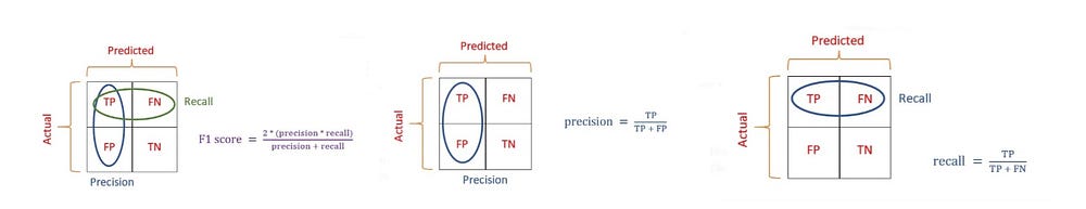
Fbeta and F2

Fbeta=(1+B^2)*(precision*recall)/(B^2*precision+recall)

the more you care about recall over precision the higher beta you should choose

F2 score, recall is twice as important to us.
confusion matrix
Result of classification:

TP FP

FN TN
- TP - ok
- TN - ok
- FP - must be negative
- FN - must be positive
- Type 1 Error - FP
- Type 2 Error - FN
metrics:
- Recall = TP / (TP + FN)
- Precision = TP / (TP + FP)
- F-Score = TP / (TP + FP)
- F-мера (F-measure) =2*(Precision*Recall)/(precision+recall) =1/(a1/precision+(1-a)/recall), a∈[0,1] - задаёт соотношение весов точности и полноты
print("accuracy\t%f" % (np.round(ypred2) = labels_test).mean()) print("loss\t\t%f" % (np.round(ypred2) ! labels_test).mean())

sklearn.metrics.classification_report(labels_test, np.round(ypred2)) # all

TP	FP
FN	TN

AUC ROC Curve

AUC-ROC (Area Under Curve - Receiver Operating Characteristics) curve - is the model selection metric for bi-milti class classification problem,

ROC curve

False Positive Rate (FPR) on the X-axis (
True Positive Rate (TPR) on the Y-axis
tells us how good the model is for distinguishing the given classes, in terms of the predicted probability.
насколько равномерно достигаются целевые классы + общее заполнение
FPR = FP / Neg(реальн) = FP / (FP + TN) - total number of negative
TPR = TP/ Pos(реальн) = TP / (TP + FN) - total number of positive

ideal value for AUC is 1 - use differentiation, hard to understand

AUC = ∫TPR d(FPR) - equal to the probability that a classifier will rank a randomly chosen positive instance higher than a randomly chosen negative one
sklearn.metrics.roc_auc_score(y_true, y_score)

pros:

good for imbalanced data

for multiclassification every class should have own curve

ROC AUC score is equivalent to calculating the rank correlation between predictions and targets. From an interpretation standpoint, it is more useful because it tells us that this metric shows how good at ranking predictions your model is. It tells you what is the probability that a randomly chosen positive instance is ranked higher than a randomly chosen negative instance.

What is

curve

           0-class precision
     ^          ... ./
     |        ..   /
     |     ...   /
TPR(1)    .    /
     |    .  /
     |  .  /
     | . /
     |./
     |/----------------->
             FPR

illustration of ROC

sklearn example

roc_auc_score == auc

from sklearn.datasets import make_classification
from sklearn.linear_model import LogisticRegression
from sklearn.model_selection import train_test_split
from sklearn.metrics import roc_curve, auc
from sklearn.metrics import roc_auc_score
from matplotlib import pyplot as plt
# генерируем датасет на 2 класса
X, y = make_classification(n_samples=1000, n_classes=2, random_state=1)
# разделяем его на 2 выборки
trainX, testX, trainy, testy = train_test_split(X, y, test_size=0.5, random_state=2)
# обучаем модель
model = LogisticRegression(solver='lbfgs')
model.fit(trainX, trainy)
# получаем предказания
lr_probs = model.predict_proba(testX)
# сохраняем вероятности только для положительного исхода
lr_probs = lr_probs[:, 1]
# рассчитываем ROC AUC
lr_auc = roc_auc_score(testy, lr_probs)
print('LogisticRegression: ROC AUC=%.3f' % (lr_auc))
# рассчитываем roc-кривую
fpr, tpr, treshold = roc_curve(testy, lr_probs)
roc_auc = auc(fpr, tpr)
# строим график
plt.plot(fpr, tpr, color='darkorange',
         label='ROC кривая (area = %0.2f)' % roc_auc)
plt.plot([0, 1], [0, 1], color='navy', linestyle='--')
plt.xlim([0.0, 1.0])
plt.ylim([0.0, 1.05])
plt.xlabel('False Positive Rate')
plt.ylabel('True Positive Rate')
plt.title('Пример ROC-кривой')
plt.legend(loc="lower right")
plt.show()

Gini coefficient, Gini impurity index, G1
- https://habr.com/ru/company/ods/blog/350440/
- https://dyakonov.org/2015/12/15/%D0%B7%D0%BD%D0%B0%D0%BA%D0%BE%D0%BC%D1%8C%D1%82%D0%B5%D1%81%D1%8C-%D0%B4%D0%B6%D0%B8%D0%BD%D0%B8/
- https://github.com/oliviaguest/gini
- В ML - метрика качества, которая часто используется при оценке предсказательных моделей в задачах бинарной
классификации в условиях сильной несбалансированности классов целевой переменной. how good the model is for distinguishing the given classes
- Обычный коэффициент Джини идеального алгоритма всегда будет равен 0.25
- Gperfect = 0.25
- Gnorm = Gmodel/Gperfect
gini_normalized = 2 * roc_auc_score(actual, predict) - 1
- Предсказание идеального алгоритма является максимальным коэффициентом Джини для текущего набора данных и зависит только от истинного распределения классов в задаче.
- Коэффициент Джини случайного алгоритма равен 0
- Значения нормализованного коэффициента Джини для обученного алгоритма находятся в интервале [0,1]
Gini = (AUC-0.5)/0.5 = 2*AUC - 1
- (AUC - 0.5) площадь верхнего треугольника
- /0.5 делить на площадь нижнего треугольника
G1 = 1 - ∑(Xk - X(k-1))*(Yk + Y(k-1))

Gini — то насколько «заполнена» верхняя половина квадрата, т.е. отношение площади над диагональю, к площади треугольника под диагональю

Example:
- accuracy 0.934783
- auc 0.84375
- gini 0.6875
- 0.0 0.98 precision
- 1.0 0.33 precision
- (0.98 + 0.33) /2 = 0.655
```
# without scikit-learn
def gini(actual, pred, cmpcol = 0, sortcol = 1):
    assert( len(actual) == len(pred) )
    all = np.asarray(np.c_[ actual, pred, np.arange(len(actual)) ], dtype=np.float)
    all = all[ np.lexsort((all[:,2], -1*all[:,1])) ]
    totalLosses = all[:,0].sum()
    giniSum = all[:,0].cumsum().sum() / totalLosses

    giniSum -= (len(actual) + 1) / 2.
    return giniSum / len(actual)

def gini_normalized(a, p):
    return gini(a, p) / gini(a, a)
```
1. В экономике
  Показатель степени расслоения общества относительно какого-либо экономического признака - 0-1 или 0-100%
  
  G = 1-[n]∑(Xk-X[k-1])*(Yk+Y[k-1])
  - n - число жителей
  - Xk - кумулятивная доля населения
  - Yk - кумулятивная доля дохода
  7 человек получают 1 рубль в год, 1 человек — 10 рублей, 1 человек — 33 рубля и один человек — 50 рублей, суммарный доход = 100
  - n = 10
  - Xk = [1-n]∑k/n = np.cumsum(np.ones(10)/10) 0.1 0.2 0.3 0.4 0.5 0.6 0.7 0.8 0.9 1.0
  - Xk-1 = 0. , 0.1, 0.2, 0.3, 0.4, 0.5, 0.6, 0.7, 0.8, 0.9
  - Yk = ∑kД/сумма = [0.01,0.02,0.03,0.04,0.05,0.06,0.07,0.17,0.50,1.00]
```
import numpy as np
x = np.cumsum(np.ones(10)/10)
xk_1 = np.roll(x,1)
xk_1[0] = 0
y = [0.01,0.02,0.03,0.04,0.05,0.06,0.07,0.17,0.50,1.00]
yk_1 = np.roll(y,1)
yk_1[0] = 0
```
  np.sum((x - xk_1) * (y + yk_1))
2. В ML
  - https://habr.com/en/company/ods/blog/350440/
  бинарная классификации для 15 объектов:
```
actual = [1, 1, 1, 1, 1, 1, 0, 0, 0, 0, 0, 0, 0, 0, 0]
predict = [0.9, 0.3, 0.8, 0.75, 0.65, 0.6, 0.78, 0.7, 0.05, 0.4, 0.4, 0.05, 0.5, 0.1, 0.1]

data = zip(actual, predict)
sorted_data = sorted(data, key=lambda d: d[1], reverse=True)
sorted_actual = [d[0] for d in sorted_data] #actual sorted by predict descending

cumulative_actual = np.cumsum(sorted_actual) / sum(actual)
cumulative_index = np.arange(1, len(cumulative_actual)+1) / len(predict) #or np.cumsum(np.ones(15)/15)
cumulative_actual_perfect = np.cumsum(sorted(actual, reverse=True)) / sum(actual) #sort actual by descending

x_values = [0] + list(cumulative_index)
y_values = [0] + list(cumulative_actual)
y_values_perfect = [0] + list(cumulative_actual_perfect)

f1, f2 = interp1d(x_values, y_values), interp1d(x_values, y_values_perfect) #функции по точкам
S_pred = quad(f1, 0, 1, points=x_values)[0] - 0.5 # площадь - Джини для модели
S_actual = quad(f2, 0, 1, points=x_values)[0] - 0.5 # площадь - джини для идеала
G = S_pred/ S_actual # коэффициент Джини
```

K-S Kolomogorov Smirnov

a measure of the degree of separation between the positive and negative distributions.

-> Rank the N random numbers in ascending order. -> Calculate D+ as max(i/N-Ri) for all i in(1, N) -> Calculate D- as max(Ri-((i-1)/N)) for all i in(1, N) -> Calculate D as max(D+, D-) -> If D>D(alpha) Rejects Uniformity else It fails to reject the Null Hypothesis.

import random

N = int(input("Enter the size of random numbers to be produced : "))
D_plus =[]
D_minus =[]
_random =[]

# Rank the N random numbers
for i in range(0, N):
    _random.append(random.random())
    _random.sort()

# Calculate max(i/N-Ri)
for i in range(1, N + 1):
    x = i / N - _random[i-1]
    D_plus.append(x)

# Calculate max(Ri-((i-1)/N))
for i in range(1, N + 1):
    y =(i-1)/N
    y =_random[i-1]-y
    D_minus.append(y)

# Calculate max(D+, D-)
ans = max(max(D_plus, D_minus))
print("Value of D is :")
print(ans)

k-fold cross validation

is the gold-standard for evaluating the performance of a machine learning algorithm on unseen data with k set to 3, 5, or 10.
R^2 Pirson - r2_score - Coefficient of determination

for regression

Измеряет совместные колебания предсказаний и меток от их средних значений, нормализованных своими соответствующими диапазонами колебаний.
Matthews Correlation Coefficient (MCC)
- for the classification problems
- MCC is a metric that considers all possibilities of binary classification (TP, TN, FP, and FN)
- robust to unbalanced datasets
- between -1 and 1
  - -1 more mistakes
  - 0 classifier is just predicting the most frequent class
MCC = (TP*TN - FP*FN)/sqrt((TP+FP)*(TP+FN)*(TN+FP)*(TN+FN))
TODO
- Статистика Колмогорова-Смирнова (вычисляется как максимальная разница между кумулятивными функциями распределения «плохих» и «хороших» заемщиков. Выше в статье приводился рисунок с распределениями и этой статистикой)
- Коэффициент дивергенции (представляет собой оценку разницы математических ожиданий распределений скоринговых баллов для «плохих» и «хороших» заемщиков, нормализованную дисперсиями этих распределений. Чем больше значение коэффициента дивергенции, тем лучше качество модели.)
Не знаю как обстоят дела в России, хоть и живу здесь, но в Европе наиболее широко применяется коэффициент Джини, в Северной Америке — статистика Колмогорова-Смирнова.
ranged based metrids
- Range-based Recall & Precision (RR,PR)
- Time-Series Aware Precision and Recall(TaP,TaR)
article "A Study on Performance Metrics for Anomaly Detection Based on Industrial Control System Operation Data"

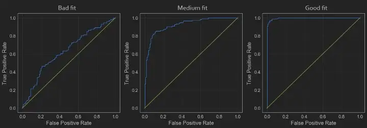
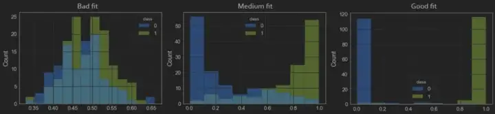
9.6.35. forecast

y - actual, x - forecasted

Mean forecast error - mean(y-x) - one value - ~0 - good
Mean absolute error - mean(|mfe|/x) - one value

Рост или падение за период p: (p.mean() - p[0])/p[0] - [-1 …. ∞]

https://facebook.github.io/prophet/

9.6.36. Machine Learning Crash Course Google https://developers.google.com/machine-learning/crash-course/ml-intro

Terms:

overfitting - хорошо на обучающей, плохо на новых
underfitting - возможно плохая модель
Kernel method or kernel trick - computing the inner products between the images of all pairs of data in implicit, high-dimensional feature space without ever computing the coordinates of the data in that space
outliers - Values distant from most other values
- Weights with high absolute values
- Predicted values relatively far away from the actual values
- Input data whose values are more than roughly 3 standard deviations from the mean.
clipping - handling outliers - Clip all values over 60 to be exactly 60 - Clip all values under 40 to be exactly 40

Когда признаков слишком много, то легко переобучить

Machine Learning is an algorithm that can learn from data without relying on rules-based programming.

describing your data with features a computer can understand
learning algorithm - Optimizing the weights on features

Statistical Modelling is formalization of relationships between variables in the form of mathematical equations.

Deep Learning - (dominant model - neural networks) - похожа на stacked logistic regression (Mathematical statistics) - uses multiple layers to progressively extract higher level features from the raw input

representation learning - automatically learn good features
Deep learning algorithms - to learn (multiple levels of) representation and an output
from raw input - sound, characters, words

few-shot learning algorithms - used when training data becomes costly

semi-supervised manner with unlabeled images - produce new data - add random noise
Parameter-level approach - parameter space can be limited - regularization techniques or loss functions are often employed

9.6.37. Дилемма смещения–дисперсии Bias–variance tradeoff or Approximation-generalization tradeoff

The bias error Смещение is an error from erroneous assumptions in the learning algorithm. How well model fit to training data.

erroneous assumptions - ошибочные заключения
very small training error -> very small bias
bias is a way of describing the difference between the actual, true relationship in our data

The variance Дисперсия is an error from sensitivity to small fluctuations in the training set.

how consistent a certain machine learning model is in its predictions when compared across similar datasets
small fluctuation of the error -> small variance
model performs poorly, and does so consistently. - small variance

Training	Validation
high bias	low variance	underfitting
low bias	high variance	overfitting

also

Models with high bias will have low variance.
Models with high variance will have a low bias.

model complexity

variance
      |
      |                 |
       \               /-------bias
        \_           _/
          \__     __/
   ----------\---/-------------------> Model complexity

Algorithms

Algorithm	Bias	Variance
Linear Regression	High Bias	Less Variance
Decision Tree	Low Bias	High Variance
Bagging	Low Bias	High Variance (Less than Decision Tree)
Random Forest	Low Bias	High Variance (Less than Decision Tree and Bagging)

9.6.38. Explainable AI (XAI) and Interpretable Machine Learning (IML) models

2020 book https://christophm.github.io/interpretable-ml-book/
https://christophm.github.io/interpretable-ml-book/
Interpretable Machine Learning with Python http://savvastjortjoglou.com/intrepretable-machine-learning-nfl-combine.html#Feature-Contributions
2021 https://www.ambiata.com/blog/2021-04-12-xai-part-1/

terms
- narrative [ˈnærətɪv]
- We torcher our data - обрабатываем наши данные
SHAP (SHapley Additive exPlanations)
- doc https://shap.readthedocs.io/en/latest/index.html
- git https://github.com/slundberg/shap
- wiki https://ru.wikipedia.org/wiki/%D0%92%D0%B5%D0%BA%D1%82%D0%BE%D1%80_%D0%A8%D0%B5%D0%BF%D0%BB%D0%B8
- An introduction to explainable AI with Shapley values https://shap.readthedocs.io/en/latest/example_notebooks/overviews/An%20introduction%20to%20explainable%20AI%20with%20Shapley%20values.html
Shapley value (Вектор Шепли)- how important is each player to the overall cooperation, and what payoff can he or she reasonably expect? The Shapley value provides one possible answer to this question.

SHAP – значения интерпретируют влияние определенного значения признака в сопоставлении с прогнозом, которое мы сделали бы, если бы этот признак принял бы некоторое базовое значение.
- value function
- Shapley value для каждого игрока - его вклад и мера выигрыша
- the SHAP value for a specific feature is just the difference between the expected model output and the partial dependence plot at the feature’s value
- SHAP values of all the input features will always sum up to the difference between baseline (expected) model output and the current model output for the prediction being explained.
- SHAP values are sensitive to high correlations among different features.
- SHAP values represent a descriptive approximation of the predictive model
- each individual rows will have their own set of SHAP values ( for customer)
- SHAP value of a feature represents the impact of the evidence provided by that feature on the model’s output
steps
1. create Explainer(model)
2. .shap_values(X) - Estimate the SHAP values for a set of samples - matrix # samples # features
1. theory
  
  KernelSHAP. This method works by permuting feature values and making predictions on those permutations. Once we have enough permutations, the Shapley values are estimated using linear regression
2. shap_values
  
  shape (rows,features)
3. supported algorithms:
  - TreeExplainer: Support XGBoost, LightGBM, CatBoost and scikit-learn models by Tree SHAP.
  - DeepExplainer (DEEP SHAP): Support TensorFlow and Keras models by using DeepLIFT and Shapley values.
  - GradientExplainer: Support TensorFlow and Keras models.
  - KernelExplainer (Kernel SHAP): Applying to any models by using LIME and Shapley values.
  - “permutation”
  - “partition” - explain the output of any function.
  - “tree”
  - “kernel” - special weighted linear regression to compute the importance of each feature
  - “sampling” - It is a good alternative to KernelExplainer when you want to use a large background set (as opposed to a single reference value for example).
  - “linear”
  - “deep” - for deep learning models
  - “gradient”
  Explainer - auto LinerExplainer TreeExplainer DeepExplainer KernelExplainer PartitionExplainer PermutationExplainer SamplingExplainer AdditiveEplainer GPUTreeExplainer GradientExplainer
4. expected_value
  property of Explainer - average model output over dataset
  - model.predict(data).maan(0) - средняя в столбце, если y - список - это число
  feature pushed value higher - red, lower - blue
5. interaction values
  https://h1ros.github.io/posts/explain-the-interaction-values-by-shap
  
  square for every record - numpy.ndarray
  
  main effects are on the diagonal and the interaction effects are off-diagonal
  
  SHAP interaction values are a generalization of SHAP values to higher order interactions.
  1. summary plot
  2. dependece plot for 2 features
6. plot
  - bar
    - single row of ShapV - shap value as a bar chart
    - multi-row of ShapV - mean absolute value for each feature column as a bar chart
  - waterfall - one-dimensional Explanation object - explantion of a single prediction as a waterfall plot
  - scatter - column of SHAP - shap_values[:,”Feature A”] - value of the feature on the x-axis, SHAP value on y-axis
    - shap.plots.scatter(shap_values[:,"RM"], color=shap_values) - e SHAP value of that feature vs. the value of the feature for all the examples in a dataset. If we pass the whole explanation tensor to the color argument the scatter plot will pick the best feature to color by.
  - heatmap - multi-row ShapV - ?
  - force -
    - single row of ShapV - waterfall in ine line
    - multi-row of ShapV - single rows rotated by 90 degree and stacked together
  - text
  - image
  - partial_dependence
  - beeswarm - used as summary plot
  - decision
  SHAP Summary Plot https://shap-lrjball.readthedocs.io/en/latest/generated/shap.summary_plot.html
  - feature importance with magnitude by classes
    - beeswarm - dots - instances and its densities. Color is used to display the original value of a feature
      
      default the features are ordered using shap_values.abs.mean(0)
  SHAP Dependence Plots -
7. limitations
  - we assume feature independence - not correlated
  - not for causal inference -
    - Shap is not a measure of “how important a given feature is in the real world”, it is simply “how important a feature is to the model”. — Gianlucca Zuin
  - human error - Confirmation bias —unconsciously favoring information that confirms your previously existing beliefs
Model-Agnostic Interpretation Methods
- Partial Dependence Plot (PDP)
Model-specific Interpretation Methods

false positive

gini1 = []

res21 = []
res22 = []
res23 = []
res24 = []

acc2 = []
gini2 = []
def run():
    for train_index, test_index in skf.split(X, Y):
        X_train, X_test = X.iloc[train_index, :], X.iloc[test_index, :]
        Y_train, Y_test = Y.iloc[train_index, :], Y.iloc[test_index, :]

        # Обучаем на фолде отклоненных андерайтером
        dtrain = xgb.DMatrix(X_train, Y_train['under']) # under
        bst: Booster = xgb.train(param, dtrain, num_round)

        # Тестируем на отклоненных системой
        dtest = xgb.DMatrix(X_test, Y_test['system']) # system
        ypred2: np.array = bst.predict(dtest)

        cn = []
        cp = []
        for i, x in enumerate(Y_test['system']):
            if x == 0:
                cn.append(ypred2[i])
            if x == 1:
                cp.append(ypred2[i])
        res21.append((np.round(cn) == 0).mean())
        res22.append((np.round(cn) == 1).mean())
        res23.append((np.round(cp) == 1).mean())
        res24.append((np.round(cp) == 0).mean())
        acc1.append((np.round(ypred2) == Y_test['system']).mean())
        auc = sklearn.metrics.roc_auc_score(Y_test['system'], ypred2)
        gini1.append(2 * auc - 1)


        # тестируем на отклоненных андерайтором
        dtest = xgb.DMatrix(X_test, Y_test['under'])
        ypred2: np.array = bst.predict(dtest)

        cn = []
        cp = []
        for i, x in enumerate(Y_test['under']):
            if x == 0:
                cn.append(ypred2[i])
            if x == 1:
                cp.append(ypred2[i])
        res1.append((np.round(cn) == 0).mean())
        res2.append((np.round(cn) == 1).mean())
        res3.append((np.round(cp) == 1).mean())
        res4.append((np.round(cp) == 0).mean())
        acc2.append((np.round(ypred2) == Y_test['under']).mean())
        auc = sklearn.metrics.roc_auc_score(Y_test['under'], ypred2)
        gini2.append(2 * auc - 1)

    print("Результаты кросс-валидации тестирования на отклоненных системой")
    print("Точность:", np.array(acc1).mean())
    print("Коэффициент gini:", np.array(gini1).mean())
    print("TrueNegative/Negative для 0:\t%f" % np.array(res21).mean())
    print("FalsePositive/Negative для 0:\t%f" % np.array(res22).mean())
    print("TruePositive/Positive для 1:\t%f" % np.array(res23).mean())
    print("FalseNegative/Positive для 1:\t%f" % np.array(res24).mean(), "\n")

    print("Результаты кросс-валидации тестирования на отклоненных андерайтором")
    print("Точность:", np.array(acc2).mean())
    print("Коэффициент gini:", np.array(gini2).mean())
    print("TrueNegative/Negative для 0:\t%f" % np.array(res1).mean())
    print("FalsePositive/Negative для 0:\t%f" % np.array(res2).mean())
    print("TruePositive/Positive для 1:\t%f" % np.array(res3).mean())
    print("* FalseNegative/Positive для 1:\t%f" % np.array(res4).mean())

9.7. Sampling

drawing random samples form statistical distibution to have constant distribuion.

Slice sampling - simplest techniques - require that distribution to be sampled be evaluable.
Markov chain Monte Carlo (MCMC)
rejection sampling

9.7.1. slice sampling

Choose a starting value x0 for which f(x0) > 0.
Sample a y value uniformly between 0 and f(x0).
Draw a horizontal line across the curve at this y position.
Sample a point (x, y) from the line segments within the curve.
Repeat from step 2 using the new x value.

9.8. likelihood, the log-likelihood, and the maximum likelihood estimate

9.8.1. links

https://en.wikipedia.org/wiki/Likelihood_function

9.9. Reinforcement learning (RL)

9.9.1. terms

Stochastic stəˈkæstɪk refers to the property of being well described by a random probability distribution.
Optimal control or just - is a branch of mathematical optimization that deals with finding a control for a dynamical system over a period of time such that an objective function is optimized.
optimal control theory
control is a variable chosen by the controller or agent to manipulate state variables, similar to an

actual control valve.

state variable is one of the set of variables that are used to describe the mathematical "state" of a dynamical system.
Phase space Фазовое пространство or state space - space in which all possible "states" of a

dynamical system or a control system are represented.

Control system - manages, commands, directs, or regulates the behavior of other devices or systems using control loops.
Dynamical system - is a system in which a function describes the time dependence of a point in an

ambient space, such as in a parametric curve.

agent - Software programs that make intelligent decisions and they are the learners in RL. These agents interact with the environment by actions and receive rewards based on there actions.
environment - is typically stated in the form of a Markov decision process (MDP)
transition - Moving from one state to another
Conditional probability distribution of Y given X, P(Y|X), is the probability distribution of Y when X is known to be a particular value. may be expressed as functions containing the unspecified value x.
return - total sum of reward the agent receives from the environment = r1+r2+r3, where 1,2,3 is states.

9.9.2. basic

area of machine learning concerned with how intelligent agents ought to take actions in an environment in order to maximize the notion of cumulative reward

RL is a basic machine learning paradigms, alongside supervised learning and unsupervised learning.
focused on finding a balance between exploration (of uncharted territory) and exploitation (of current knowledge).

9.9.3. environment is typically stated in the form of a Markov decision process (MDP)

S - environment and agent state space
A - set of actions
P(s,s') - probability of transtion from s to s' under action a.
R(s,s') - reward after transition

observability

full - agent observes the current environmental state
partial - with noise or not full

Problems:

model of the environment is known (planning problem)
simulation model of the environment (planning problem)
only way to collect information about the environment is to interact with it

trade-offs

long-term versus short-term reward trade-off
The exploration vs. exploitation trade-off

9.9.4. Dynamic programming

DP is both a mathematical optimization method and a computer programming method.

If sub-problems can be nested recursively inside larger problems, so that dynamic programming methods are applicable.

There is a relation between the value of the larger problem and the values of the sub-problems. In the optimization literature this relationship is called the Bellman equation.

9.9.5. Markov decision process (MDP)

Markov decision process (MDP) - is a discrete-time stochastic 2 process. It provides a mathematical framework for modeling decision making in situations where outcomes are partly random and partly under the control of a decision maker.

MDPs are useful for studying optimization problems solved via dynamic programming.

type (S, A, P, R, γ) - Markov decision process

S - state space, anything which can be useful in choosing actions. the statespace of the process is constant through time.
A - action space (alternatively, A is set of actions available from state s)
P(s, s') - is a probability that action a in state s at time t will lead to state s' at time t+1.
R(s, s') - immediate reward (or expected immediate reward) received after transitioning from state s to state s', due to action a.
γ - discount factor that is used to reduce the importance of the of future rewards. (optional)

reward calculation is considered to be the part of the environment

policy function π is is a (potentially probabilistic) mapping from state space S to action space A.

The goal in a Markov decision process is to find a good "policy" for the decision maker: a function π that specifies the action π(s) that the decision maker will choose when in state s.

Markov property refers to the memoryless property of a stochastic process. conditional probability distribution of future states of the process (conditional on both past and present values) depends only upon the present state.

classes of Markov process are the Markov chain and the Brownian motion.

Discount Factor (ɤ) - helps us to avoid infinity as a reward in continuous tasks.

0 - more importance is given to the immediate reward.
1 - more importance is given to future rewards
return G(t) = R(t+1) + ɤ*R(t+2) + ɤ^2*R(t+3) + …

Value Function determines how good it is for the agent to be in a particular state.

Bellman Equation for Value Function: v(s) = E[(R(t+1) + ɤ*v(S(t+1))) | St=s]
- Immediate Reward of successor states + Discounted value of successor states.

policy defines what actions to perform in a particular state s. defines a probability distribution over Actions (a∈ A) for each state (s ∈ S) at. π(a|s) is the probability that the agent with taking action (a ) at a particular time step (t). π(a|s) = P[At=a|St=s]

methods to solve:

Dynamic Programming (Value iteration and Policy iteration)
Monte-Claro methods
TD-Learning.

State-action value function or Q-Function - how good it (value) is for the agent to take action (a) in a state (s) with a policy π.

9.9.6. Markov chain

type of Markov process that has either a discrete state space or a discrete index set (often representing time), but the precise definition of a Markov chain varies.

9.9.7. links

https://en.wikipedia.org/wiki/Reinforcement_learning
https://towardsdatascience.com/introduction-to-reinforcement-learning-markov-decision-process-44c533ebf8da
Recurrent Policy Gradients 2009 Юрген Шмидхубер https://mediatum.ub.tum.de/doc/1287506/file.pdf

9.10. Distributed training

9.10.1. temrs

offloading - offload the sharded model parameters to CPUs.
Half-Precision - float16

9.10.2. all

GPU cluster concept - each node is equipped with a Graphics Processing Unit (TPU clusters that are more powerful than GPU clusters.)

types of distributed training:

Data parallelism (many copies of model) - not for large models
Model parallelism (split model, all worker nodes use the same dataset)
- neural network model should have a parallel architecture
- hard to implement
- параллелизм моделей чаще всего используется в сфере обработки естественных языков, в моделях, где
используются трансформеры, в таких проектах, как GPT-2, BERT, и в других подобных.
GPU parallelism - several GPUs in one computer

Synchronization methods:

parameter server technique - dividing all GPU nodes into two groups
- if the global model parameters are synchronously shared across workers, you will wait until each worker
completes its iteration and returns the results which might be time-consuming
- if you have only one parameter server, you will not benefit from adding more workers as your server will
have to work with more data from the workers which creates a bottleneck.
an all-reduce technique - allows to add more workers without any limitations (used more often than a parameter server-based architecture)
- tensorflow By default, uses the NVIDIA Collective Communication Library (NCCL) as the all-reduce implementation.

tools:

NCCL and MPI (Message Passing Interface) - параллелизм модели - на каждом кусок сети.
- Horovod - distributed training framework for TensorFlow, Keras, PyTorch, and MXNet
- Gloo - Pytorch
- NVCaffe - Caffe
Parameter server (PS) - параллелизм данных - на каждом полная модель
Model Parallelism for tensorflow https://github.com/tensorflow/mesh

Scalability:

t1 - time to complete
N processing elements
tN - amount of time to complete with N processors
Strong Scaling = t1 / ( N * tN ) * 100%
Weak scallig - constant and additional elements are used to solve a larger total problem (one that wouldn't fit in RAM on a single node = ( t1 / tN ) * 100%

Automatic loss scaling - improve stability when training large models in mixed precision. Lower precision numerical formats introducing numerical instabilities during training, reducing the statistical performance of some models, potentially hampering statistical convergence. (https://arxiv.org/pdf/2112.11446.pdf). ALS aims to shift the gradient distribution across the dynamic range, so that underflow and overflow are prevented (as much as possible) in float-16.

loss scaling is not needed for some networks (e.g. image classification, Faster R-CNN), but necessary for others (e.g. Multibox SSD, big LSTM language model).

Automatic Mixed Precision (AMP) - is the same as with fp16, except it'll use bf16. Nvidia.

Converting the model to use the float16 data type where possible.
Keeping float32 master weights to accumulate per-iteration weight updates.
Using loss scaling to preserve small gradient values.
https://docs.nvidia.com/deeplearning/performance/mixed-precision-training/index.html
https://nvidia.github.io/apex/amp.html

Distributed Data Parallel (DDP) - short: per-GPU copy of a model’s parameters, gradients and optimizer states. long: Applications using DDP should spawn multiple processes and create a single DDP instance per process. DDP registers an autograd hook for each parameter given by model.parameters() and the hook will fire when the corresponding gradient is computed in the backward pass. Then DDP uses that signal to trigger gradient synchronization across processes. (GPU devices cannot be shared across processes)

Fully Sharded Data Parallel (FSDP) - shards model’s parameters, gradients and optimizer states across data-parallel workers and can optionally offload the sharded model parameters to CPUs.

9.10.3. tips

When solving a deep learning problem GPU is more powerful than CPU
A CPU is good in the tasks where latency or per-core performance is important
CUDA is a tool that is used to communicate with a GPU
cuDNN is the library that is optimized for working on GPUs and has highly tuned implementations for standard deep learning routines. cuDNN provides highly tuned implementations for standard routines such as forward and backward convolution, pooling, normalization, and activation layers.

9.10.4. paradigms

9.10.5. links

comparision of distributed ml systems https://arxiv.org/pdf/1909.02061.pdf
article GOOD https://lilianweng.github.io/posts/2021-09-25-train-large/
https://huggingface.co/docs/transformers/v4.17.0/en/parallelism

9.11. Federated learning (or collaborative learning)

distributed learning originally aims at parallelizing computing power, training a single model on multiple servers
federated learning - aims at training on heterogeneous datasets

9.12. Statistical classification

categories - classes
observations - instances in machine learning
properties of observations - features (grouped into a feature vector)
training set - observations (or instances) whose category membership is known
Classification is an example of pattern recognition.
supervised learning
unsupervised procedure is known as clustering
Унитарный код (one-hot) - двоичный код фиксированной длины, 1 - прямой - 000010, Инверсный - 111101

9.12.1. in satistics

used logistic regression
properties of observations = explanatory variables (or independent variables, regressors, etc.)
categories to be predicted are known as outcomes - dependent variable

9.13. Тематическое моделирование

к каким темам относится каждый документ коллекции

9.14. Популярные методы

https://tproger.ru/translations/top-machine-learning-algorithms/
Cluster analysis - упорядочивающая объекты в сравнительно однородные группы
Collaborative filtering - это один из методов построения прогнозов (рекомендаций) в рекомендательных системах[⇨], использующий известные предпочтения (оценки) группы это один из методов построения прогнозов (рекомендаций) в рекомендательных системах[⇨], использующий известные предпочтения (оценки) группы

9.15. прогнозирование

временной ряд с аппроксимацией

9.16. Сейчас

крупные компании в какой-то мере монополизировали машинное обучение

вычислительные ресурсы и доступ к массивам данных

9.16.1. примеры

прогнозирования температуры поверхности дороги

погодные станции на автомагистралях
прогноз от Росгидромета

спрос на смартфоны

прогноз спрос производителий смартфонов на детали
прогноз спроса на детали всеми компаниями
зависимости между различными номенклатурами деталей

лидары (лазерные радары) - в пространстве ориентируются самоуправляемые автомобили ???

Яндекс-такси look-alike-модели - предлагаем ее тем, кому это будет интересно

9.16.2. библиотеки

Non distributed
- Batch
  - R language - visualisation features, which is essential to explore the data, package for machine learning
  - Python - scikit-learn
  - Weka - Java - GPL
- Stream
  - MOA (Massive On-line Analysis) Java -GPL- is a framework for data stream mining
Distributed
- Batch
  - Apache Hadoop (həˈduːp) -Java- GPL => Mahout -Java, Scala- -GPL- collaborative filtering, classification, cluster analysis
- Stream
  - (Apache S4, Storm) => SAMOA

9.17. kafka

https://dzone.com/articles/5-machine-learning-trends-2018-combined-with-apach

machine learning lifecycle:

Model training - analytic model - we feed historical data - continuous
Generating predictions - use an analytic model for making prediction - within an application or microservice

May be used with Kafka:

TensorFlow Java API, KSQL - streaming SQL

9.18. в кредитных орг-ях

Сбербанк, ВТБ - предсказательной силы показатель Джини (Gini)

Традиционные

оценка кредитных рисков
безопасность и противодействие мошенничеству
вторичные и кросс-продажи

Новые

бот-клиент
предиктивной аналитики
оптимизации бизнес-процессов
сокращения издержек и повышения уровня STP
когнитивных вычислений, благодаря которому, в краткосрочной перспективе, банк сможет вывести на рынок совершенно новые продукты и услуги, улучшить клиентский опыт и развить новые направления бизнеса

9.19. TODO Сбербанк проекты

Сбербанк использует стандарт CRISP или Cross-Industry Standard Process for Data Mining/ Data Science, определяющий, что каждая разработка roll out-модели должна идти согласно заданному жизненному циклу

9.20. KDTree simular

9.21. Применение в банке

Payment:

Reducing payment fraud
Reducing false positives
Anti-money layndery
Conversational payments

Backend:

Automating existing processes
Aiding CSRs(back end) - Корпоративная социальная ответственность - добровольно принимают дополнительные меры для повышения качества жизни работников и их семей, а также местного сообщества и общества в целом
Pre-empting problems

Front-end:

Securing dogital identity banking
- Video, fingerprints, palm recognition, voice, радужной оболочке глаза, face
Auto-saving and recommendations
Aiding CSRs
Improving iteractions across channels

Рекомендательная система - типа кал цента
- интент - вопросы пользователей -
  - поиск
  - технический вопрос
  - отзыв
  - котика запостил
- Именованные сущности в банке - продукт, свойство, величина
оптимизации обработки транзакций
кибербезопасности с выявлением мошенничества
персональных финансовых ассистентов и сверх-таргетированного маркетинга
детектируем паттерны поведения клиентов по транзакциям
- 1 предложить ему продукты или услуги, полезные для автовладельцев
- 2 предсказывать те или иные события, в том числе сам факт покупки
мы видим, кто из клиентов банка копит деньги, помогаем формировать для них новые предложения
NLP - 1 создание библиотеки правил для извлечения сущностей
- 2 семантический анализатор текста

9.22. вспомогательные математические методы

Softmax - многомерный сигмойд, преобразовывает вектор в вектор q(z)i = e^zi/∑e^zk. Координата q трактуется как вероятность того, что объект принадлежит к классу i. Область значений (0,1)
- np.exp([1,2,3,4])/np.sum(np.exp([1,2,3,4])) -> array([0.0320586 , 0.08714432, 0.23688282, 0.64391426])
- np.sum(np.exp([1,2,3,4])/np.sum(np.exp([1,2,3,4]))) -> 1.0
Сигмоида - q(x)=1/(1+e^-x)
- 1 / (1 + np.exp(-np.array([1,2,3,10]))) -> array([0.73105858, 0.88079708, 0.95257413, 0.9999546 ])

9.23. AutoML

Sberbank https://www.youtube.com/watch?v=jukZAtyJJ64

это процесс автоматизации сквозного процесса применения обучения машины к задачам реального мира

by hands:

сбор данных
пре-процессинг
конструктор факторов (features)
разработка ML алгоритма
выбор модели
валидация
продуктив

AutoML - генерация спецификаций моделей по выборке данных и выбор из них одной - главное автовалидация моделей - количественная оценить модельного риска (насколько выгодно инвестировать в её доработку)

Logistic Regression - дать или не дать - бинарная классификация
XGBoost - gradient boosting library - runs on major distributed environment (Hadoop, SGE, MPI)
SVM - Метод опорных векторов

9.23.1. Neuton AutoML https://neuton.ai/

Автоматический Feature engeering - различные сочетания столбцов
Feature importance for neural networks

классы задач

feature importance
ранжирование
стоп листы - выделение строк с низкой вероятностью
конверсия - выделение строк с высокой вероятностью
прогнозирование
сегментация

9.24. Известные Датасеты

Binary classification

https://www.kaggle.com/c/titanic - train.csv - Survived для каждого пассажира, обозначающий, выжил данный пассажир или нет (0 для умерших, 1 для выживших).

MNIST - объёмная база данных образцов рукописного написания цифр

SVHN dataset - It can be seen as similar in flavor to MNIST - images are of small cropped digist (over 600,000 digit images)

ImageNet - де факто стандарт сравнения CNN

rank 1 процент - accuracy - we compare if the class with the highest probability according to our network matches the real tag
rank 2 процент - we compare if one of the 5 classes with higher probation according to our network matches the real label

9.24.1. signatures

On-line Handwritten Signature Database login and password required http://biometrics.sabanciuniv.edu/susig.html

ICDAR http://www.iapr-tc11.org/mediawiki/index.php?title=Datasets_List

2009 Signature Verification Competition (SigComp2009)*
- usage https://github.com/gnbaron/signature-recognition
- http://www.iapr-tc11.org/mediawiki/index.php?title=ICDAR_2009_Signature_Verification_Competition_(SigComp2009)
ICFHR 2012 Signature Verification Competition (4NSigComp2012)
- http://www.iapr-tc11.org/mediawiki/index.php/ICFHR_2012_Signature_Verification_Competition_(4NSigComp2012)

CEDAR handwriting https://cedar.buffalo.edu/Databases/index.html

CEDAR signatures https://cedar.buffalo.edu/NIJ/data/signatures.rar

It consists of 24 genuine and forged signatures each from 55 different signers.
usage https://github.com/rmalav15/signature-recognition
usage https://github.com/uniyalvipin/signature-recognition

handwritten signatures https://www.kaggle.com/divyanshrai/handwritten-signatures

30 people
NFI-00602023 is an image of signature of person number 023 done by person 006 - This is a forged signature
NFI-02103021 is an image of signature of person number 021 done by person 021 - genuine signature.

English Writer recognition dataset (not signatures) IAM https://fki.tic.heia-fr.ch/databases/iam-handwriting-database

9.25. игрушечные датасеты toy datasets

9.25.1. line with standard deviation

import numpy
import matplotlib.pyplot as plt
import numpy as np

# LINE ----------------------------------
x = np.random.rand(100)

# Gaussian distribution N(mu,sigma ^2)
sigma = 0.1  # mean
mu = 0  # standard deviation
N = numpy.random.normal(mu, scale=sigma, size=x.shape[0])

y = np.reshape(5 * x + 2 + N, -1)

plt.plot(x, y, 'bo')
plt.show()

9.25.2. two bloabs of Gaussian distributions N(mu,sigma ^2)

import numpy
import matplotlib.pyplot as plt
import numpy as np

k
# Toy Logistic Regression Data ---------------
N = 100
# Zeros form a Gaussian centered at (-1, -1)
x_zeros = np.random.multivariate_normal(
    mean=np.array((-1, -1)), cov=.1*np.eye(2), size=(N//2,))
y_zeros = np.zeros((N//2,))
# Ones form a Gaussian centered at (1, 1)
x_ones = np.random.multivariate_normal(
    mean=np.array((1, 1)), cov=.1*np.eye(2), size=(N//2,))
y_ones = np.ones((N//2,))

x_np = np.vstack([x_zeros, x_ones])
y_np = np.concatenate([y_zeros, y_ones])

# Save image of the data distribution
plt.xlabel(r"$x_1$")
plt.ylabel(r"$x_2$")
plt.scatter(x_zeros[:, 0], x_zeros[:, 1], color="blue")
plt.scatter(x_ones[:, 0], x_ones[:, 1], color="red")
plt.title("Toy Logistic Regression Data")
plt.show()

9.25.3. cosine with standard deviation

import numpy
import matplotlib.pyplot as plt
import numpy as np


# COS(x) x in [-5,5] + N(0,1/5) ---------
x = np.array(np.arange(-5, 5, 0.1))

sigma = 0.5  # mean
mu = 0  # standard deviation
N = numpy.random.normal(mu, scale=sigma, size=x.shape[0])

y = np.reshape(np.cos(x) + N, -1)

plt.plot(x, y, 'bo')
plt.show()

После первого обучения мы всзвешиваем датасет на основе ошибок первого

9.25.4. normal distribution

with scipy

import numpy as np
from scipy.stats import norm
import matplotlib.pyplot as plt

rv = norm(loc=0, scale=1) # loc (location) or mean  = 0 , scale (squared) or variance = 1

x = norm.rvs(size=1000) # random variable

pdf = rv.pdf(x)
plt.scatter(x, pdf , color = 'red')
plt.hist(x, 30, density=True)
plt.show()

excess kurtosis of normal distribution (should be 0): -0.0024385251600711477
skewness of normal distribution (should be 0): 0.0013034391014922926

with numpy

import numpy as np
from scipy.stats import norm
import matplotlib.pyplot as plt
mu, sigma = 0, 1 # mean and standard deviation
x = np.random.normal(mu, sigma, 1000)
pdf = norm.pdf(x)
plt.scatter(x, pdf , color = 'red')
plt.show()

pdf of line

# Importing required libraries
import numpy as np
import matplotlib.pyplot as plt

# Creating a series of data of in range of 1-50.
x = np.linspace(1,50,200)

#Creating a Function.
def normal_dist(x , mean , sd):
    prob_density = (np.pi*sd) * np.exp(-0.5*((x-mean)/sd)**2)
    return prob_density

#Calculate mean and Standard deviation.
mean = np.mean(x)
sd = np.std(x)

#Apply function to the data.
pdf = normal_dist(x,mean,sd)

#Plotting the Results
plt.plot(x, pdf , color = 'red')

plt.xlabel('Data points')
plt.ylabel('Probability Density')
plt.show()

9.26. TODO Genetic algorithms

by iterating, variation and combining target parameters. Neural network training can serve as an example of such a task.

evolutionary computation is a family of algorithms for global optimization.

Soft computing is a set of algorithms

Approximate reasoning - processing information (data) through fuzzy rules
- Probablistic models
- Multivalued & Fuzzy Logics
Functional approximation / Randomized Search
- neural networks
- evolutionary algorithms.

Classical logic only permits conclusions that are either true or false. Fuzzy Logics - любые значения на отрезке [ 0 , 1 ].

links

9.27. TODO Uplift modelling

Models the incremental impact of a treatment.

uplift - usually defined as the difference in response rate between a treated group and a randomized control group. ( incremental effect )

many implement lift as the difference. (without predictive modeling)

ex.

Group	Number of Customers	Responses	Response Rate
Treated	1,000,000	100,000	10%
Control	1,000,000	50,000	5%

Here response rate uplift is 5%.

Перед созданием модели необходимо провести A/B-эксперимент , который заключается в следующем:

Часть активных пользователей продукта случайным образом делится на две группы: тестовую и контрольную.
К пользователям из тестовой группы применяются механизмы для удержания (бонусы, скидки, специальная коммуникация).
Опыт пользователей из контрольной группы не меняется.

библиотека scikit-uplift

Все базовые подходы можно разделить на два класса:

походы с применением одной модели
подходы с применением двух моделей.

одна модель обучается одновременно на двух группах, при этом бинарный флаг коммуникации выступает в качестве дополнительного признака. Каждый объект из тестовой выборки скорим дважды: с флагом коммуникации равным 1 и равным 0. Вычитая вероятности по каждому наблюдению, получим искомый uplift.

двух ML-моделей, которые будут предсказывать уход пользователей (как именно это делается, мы разбирали выше):

Модели, которая прогнозирует, что пользователь уйдет при отсутствии механизмов удержания. Для обучения этой модели нужно использовать данные из контрольной группы эксперимента.
Модели, которая прогнозирует, что пользователь уйдет при наличии механизмов удержания. Для обучения этой модели нужно использовать данные из тестовой группы эксперимента.

Две независимые модели:

Строится первая модель, оценивающая вероятность выполнения целевого действия среди клиентов, с которыми мы взаимодействовали.
Строится вторая модель, оценивающая ту же вероятность, но среди клиентов, с которыми мы не производили коммуникацию.
Затем для каждого клиента рассчитывается разность оценок вероятностей двух моделей.

Две зависимые модели (зависимое представление данных)

Две зависимые модели (перекрестная зависимость)

9.27.1. dataset

Hillstrom Dataset. Этот набор данных содержит информацию о 64000 покупателей, совершивших покупку в течение 12 месяцев.

9.27.2. customers segmentation

The Persuadables : customers who only respond to the marketing action because they were targeted
The Sure Things : customers who would have responded whether they were targeted or not
The Lost Causes : customers who will not respond irrespective of whether or not they are targeted
The Do Not Disturbs or Sleeping Dogs : customers who are less likely to respond because they were targeted

Uplift modelling provides a scoring technique that can separate customers.

9.27.3. metrics

Uplift curve (или Uplift кривая). - функция от количества объектов. В каждой точке кривой можно увидеть накопленный к этому моменту uplift.
uplift@k – размер uplift на топ k процентах выборки

9.27.4. mts

Формирование сегментов для продвижения

Look-alike: модель оценивает вероятность того, что клиент выполнит целевое действие.
Response модель: оценивает вероятность того, что клиент выполнит целевое действие при условии коммуникации.
Uplift модель: оценивает чистый эффект от коммуникации, пытаясь выбрать только тех клиентов, которые совершат целевое действие только при нашем взаимодействии. Модель оценивает разницу в поведении клиента при наличии воздействия и при его отсутствии.

Retention. решается путем прогнозирование оттока пользователей (churn prediction)

альтернативный подход к улучшению Retention с помощью ML — uplift-моделирование

https://habr.com/ru/companies/ru_mts/articles/485980/

9.28. A/B test

see math#MissingReference

9.29. Regression

Regression analysis - statistical processes for estimating the relationships between a dependent variable and one or more independent variables.

A regression model predicts continuous values.

Linear regression - finding the straight line or hyperplane that best fits a set of points, y dependent is a liner combination of parameters

сумма Остатков (Residual) – разницей между фактическим и спрогнозированным значениями, равна 0, то есть они распределены случайным образом вокруг нуля

Machine learning evaluation metrics. see

MSE - mean squared error. 1/n * ∑((at-pt)^2) where at is true y, pt - predicted y
MAE - mean absolute error 1/n * ∑|at-pt|
sMAPE
MAPE - mean absolute percentage error. 1/n * ∑ ((at-pt)/at) or 1/n * ∑ (1 - pt/at) - 0 no loss - inf big loss
MASE
MSPE
RMS
RMSE/RMSD
R2
MDA
MAD

MSE, RMSE is dependent on the scale of the data. It increases in magnitude if the scale of the error increases.

errors have physical dimensions and expressed in the units of the data under analysis (variable of interest

classifications:

scale-dependent measures (e.g. MSE, RMSE, MAE, MdAE);
measures based on percentage errors (e.g. MAPE, MdAPE, RMSPE, RMdSPE, sMAPE,

sMdAPE);

measures based on relative errors (e.g. MRAE, MdRAE, GMRAE);
relative measures (e.g. RelMAE, CumRAE);
scaled errors (e.g. MASE, RMSSE, MdASE)

Power distances which are based on mathematical expressions involving raising to power

(e.g. Euclidean, Manhattan, Mahalanobis, Heterogeneous distance);

Distances on distribution laws (probability-related) (e.g. Bhattacharya coefficient, Jensen,

Hellinger);

Correlation similarities and distances (e.g. Spearman, Kendall, Pearson);
Other similarities and distances which do not fit into the three main categories)

9.30. Similarity (ˌsiməˈlerədē/)

9.30.1. Cosine similarity, Orchini similarity, Otsuka–Ochiai similarity

the cosine of the angle between the vectors. applied to binary data.

cos θ = A*B / |A|*|B| - dot product / Euclidean magnitudes of A and B
∑(Ai*Bi)/sqrt(∑Ai^2)*sqrt(∑Bi^2)
|A| cos θ = scalar projection

always belongs to the interval [ − 1 , 1 ]

1 - proportional vectors
0 - orthogonal vectors
-1 opposite vectors

if required can be normolized to [ 0 , 1 ], cosine distance = [0, 2]

is not a true distance metric as it does not exhibit the triangle inequality property

solution: convert to angular distance or Euclidean distance.
- effective proxy for cosine distance can be obtained by L2 normalisation of the vectors (each term in each vector is first divided by the magnitude of the
vector, yielding a vector of unit length), followed by the application of normal Euclidean distance.
or: the triangular inequality that does work for angular distances can be expressed directly in terms of the cosines;

10. Artificial Neural Network and deep learning

международная конференция https://www.youtube.com/results?search_query=%23aijourney
https://developers.google.com/machine-learning/crash-course/ml-intro
https://playground.tensorflow.org
2019 course https://mlcourse.ai/
about playground https://cloud.google.com/blog/products/gcp/understanding-neural-networks-with-tensorflow-playground
сравнение https://en.wikipedia.org/wiki/Comparison_of_deep-learning_software
article basic https://colah.github.io/posts/2014-03-NN-Manifolds-Topology/
math of ANN https://medium.com/deep-math-machine-learning-ai/chapter-7-artificial-neural-networks-with-math-bb711169481b
продвинутые лекции https://www.youtube.com/watch?v=92Ctk9OzlDg
Geoffrey E. Hinton https://www.cs.toronto.edu/~hinton/

problems:

Catastrophic interference or catastrophic forgetting problem - forget previously learned information upon learning new information https://en.wikipedia.org/wiki/Catastrophic_interference
- https://en.wikipedia.org/wiki/Feedforward_neural_network
CNN and RNN tips https://stanford.edu/~shervine/teaching/cs-230/cheatsheet-deep-learning-tips-and-tricks
book MIT Press http://www.deeplearningbook.org/
механизм внимания ???
передаточная функция нейрона это сумматор и функция активации
скрытого уровня (hidden units) и нейронов-выходов (output units)
one epoch = one forward pass and one backward pass of all the training examples - чем больше epoch тем больше модель требует именно такие входные данные
batch size = the number of training examples in one forward/backward pass. The higher the batch size, the more memory space you'll need. if you have 1000 training examples, and your batch size is 500, then it will take 2 iterations to complete 1 epoch
Learning Rate = см 10.5.5
axon - отросток нейрона - выход
hyperparameter - дополнительная настройка для слоя
spatial (or temporal) dimension - пространственное или временное - 1D convolution layer (e.g. temporal convolution)
logits layer - last neuron layer - inverse of the sigmoid - from [0,1] to [-∞;+∞]
neural network - way of combining linear models. с нелинейными функциями
Линейная модель - y = xA + b A ∈ Rnxm , b ∈ Rm , x - вектор - однослойная нейросеть если все это от нелинейной функции
Функция активации - определяет выходной сигнал нейрона, который определяется входным сигналом или набором входных сигналов
Функция потерь Loss function(or cost function) - является мерой расхождения между истинным значением оцениваемого параметра и оценкой параметра. Используется как первый шаг в backward propogation
Negative Log-Likelihood(NLL) L(y)=-log(y)
dense data (e.g. audio)
masking in RNN - allows us to handle variable length inputs in RNNs - going to be used to skip any input with mask 0 by copying the previous hidden state of the cell;
waights initializations. Для разных моделей нужны разные инициализации. Нельзя нули - backward prop https://medium.com/usf-msds/deep-learning-best-practices-1-weight-initialization-14e5c0295b94

chars:

∘ Hadamard product (element-wise product) - a11*b11, a12*b12
⊕ element-wise plus
⊗ matrix multiplication

10.1. TODO flameworks

Все поддерживают прикладной интерфейс OpenMP, языки Pyton, Java и C++ и платформу CUDA. 2022

TensorFlow.
Shogun.
Sci-Kit Learn.
PyTorch.
CNTK.
Apache MXNet.
H2O.
Apple's Core ML.

2017

TensorFlow
Theano
Keras
Lasagne
Caffe
DSSTNE
Wolfram Mathematica

10.2. History

1943 The perceptron was invented in 1943 by McCulloch and Pitts
1958 Frank Rosenblatt - perceptron implementation
1962 Widrow & Hoff developed a learning procedure
1969 Perceptrons book shows limitation of Perceptrons by Marvin Minsky and Seymour Papert
1986 Backpropagation
1988 deep CNN - LeNet - for OCR http://vision.stanford.edu/cs598_spring07/papers/Lecun98.pdf
1997 Recurrent neural nerwork framework, LSTM by Schmidhuber & Hochreiter
1998 Yann LeCun Deep Network - recognize handwritten ZIP codes on mailed envelopes
2010s, benefitting from cheap, powerful GPU-based computing systems
2010 CNN - AlexNet from Amazonwas the first winner of the ImageNet
2012 ResNet - Residual block
2014 - generative adversarial network (GAN)
2015 - Tensorflow
2016 - PyTorch
2016 DenseNet CNN architecture https://arxiv.org/abs/1608.06993
2016 - DyNet Dynamic Neural Networks
2017 Transformers - encoder–decoder architecture - Google - Attention is all you need paper
2018 BERT - Google transformer-based - language modeling, next sentence prediction
2018 AttnGAN: Fine-grained text to image generation with attentional generative adversarial networks.
2018 GPT-1 OpenAI
2019 StackGAN++: Realistic Image Synthesis with Stacked Generative Adversarial Networks.
2019 EfficientNet architecture - применяется для обнаружения объектов - https://arxiv.org/abs/1905.11946
2019 Tensorflow 2.0
2020 GPT-2/3 Micorosft - autoregressive language model that uses deep learning to produce human-like text. GPT-3 – это ПО с закрытым программным кодом
2021 OpenAI company - DALL·E сеть, это версия GPT-3, генерировать изображения из текстовых описаний на датасете из пар текст-изображение
2021 SberDevices ruGPT-3 (ruDALL-E Kandinsky) с действительно, открытым кодом.
2021 CLIP, CogView
2022 Stable Diffusion, Mindjourney, Chat GPT
2023 GPT-4

ResNet, ResNext, EfficientNet, EfficientDet, SSD, MaskRCNN, Unet, VNet, BERT, GPT-2, Tacotron2 and WaveGlow

links
- https://www.tadviser.ru/index.php/%D0%A1%D1%82%D0%B0%D1%82%D1%8C%D1%8F:%D0%9C%D0%B0%D1%88%D0%B8%D0%BD%D0%BD%D0%BE%D0%B5_%D0%BE%D0%B1%D1%83%D1%87%D0%B5%D0%BD%D0%B8%D0%B5_(Machine_Learning)

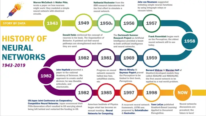
10.2.1. Перцептрон

http://neerc.ifmo.ru/wiki/index.php?title=%D0%9D%D0%B5%D0%B9%D1%80%D0%BE%D0%BD%D0%BD%D1%8B%D0%B5_%D1%81%D0%B5%D1%82%D0%B8,_%D0%BF%D0%B5%D1%80%D1%86%D0%B5%D0%BF%D1%82%D1%80%D0%BE%D0%BD
Возможности и ограничения перцептронов https://ru.wikipedia.org/wiki/%D0%92%D0%BE%D0%B7%D0%BC%D0%BE%D0%B6%D0%BD%D0%BE%D1%81%D1%82%D0%B8_%D0%B8_%D0%BE%D0%B3%D1%80%D0%B0%D0%BD%D0%B8%D1%87%D0%B5%D0%BD%D0%B8%D1%8F_%D0%BF%D0%B5%D1%80%D1%86%D0%B5%D0%BF%D1%82%D1%80%D0%BE%D0%BD%D0%BE%D0%B2
S, A, R слоя
Нейрон - покой или возбуждение - сумматор + функция активации
связь с весом.
каждый -
- сумматор of boolean inputs ∑wixi-θ (dot product of two vectors w x) θ - bias constant or threshold
- функция активации
  - threshold function 1 если ∑wixi-θ>0(or ∑wixi>θ) иначе 0. w и х - вектора

f(x) = sign(∑wixi-θ). Обучение:

Метод коррекции ошибки - метод обучения перцептрона. Сначала весы случайные, не изменяется пока правильно, если неправильно, то прибавляется или вычисляется что-то
Backpropagation метод обратного распространения ошибки "the backward propagation of errors," - метод вычисления градиента, который используется при обновлении весов многослойного перцептрона
- gradient of the loss function
- передаточная функция нейрона должна быть дифференцируема

Note:

Single layer perceptrons are only capable of learning linearly separable patterns. Два множества точек в двумерном пространстве называются линейно сепарабельными (линейно разделимыми), если они могут быть полностью отделены единственной прямой
dot product - quantifies how much one vector is going in the direction of the other

теорема о сходимости перцептрона FEC - независимо от начальных значений коэффициентов и порядка показа образцов при обучении, перцептрон за конечное число шагов научится различать два класса объектов, если только существует такая классификация

10.3. Evolution of Deep Learning

Statistical Modeling - math models and statistics based on insights and patterns observed in the data
Native Deep Learning - for every unique task, a new dataset was curated and a model was trained from scratch.
Transfer learning - even with smaller datasets, effective models could be developed by transferring knowledge.
Foundational Models - Transformers, possible to tran massive models and massive datasets, LLM.
AGI - every single task can be solved in zero-shot, without training

10.4. persons

Джефри Хинтон - Hinton - прижизненную славу классика, статьи в Nature
Ян Лекун - LeCun
Иешуа Бенджо - Bengio
Владимир Вапник
Эндрю Ын - Baidu - связал глубинное обучение с графическими процессорами
Christian S. Perone ML Research Engineer in London/UK https://blog.christianperone.com/

google

10.5. Theory basis

10.5.1. NN definition (stanford)

NN consist of Trashold Login Unit (TLU):

inputs X
weights W
activation (treshold for perceptron) function
- sum
- treshold
- bias (optional)

TLU as dot product: X*W

f(x) = 1 if w*x+b>0, 0 otherwhise

w and x is vectors
https://ai.stanford.edu/~nilsson/MLBOOK.pdf

   x1
   *\
     \
      \w1
       \         threshold
   x2 w2\       /
   *-----(∑)---[]-----> f
        /
     w3/
      /
  x3 /
   */

weights, filters

Each neuron in a neural network computes an output value by applying a specific function to the input values received from the receptive field in the previous layer. The function that is applied to the input values is determined by a vector of weights and a bias (typically real numbers). Learning consists of iteratively adjusting these biases and weights.

The vectors of weights and biases are called filters and represent particular features of the input (e.g., a particular shape). A distinguishing feature of CNNs is that many neurons can share the same filter. This reduces the memory footprint because a single bias and a single vector of weights are used across all receptive fields that share that filter, as opposed to each receptive field having its own bias and vector weighting.

10.5.2. activation functions

∇ - nabla, gradient, pronounced "del", vector differential operator - result is a vector of partial derivatives

types:

saturating if lim->inf |∇f(u)| = 0
nonstaturating, such as ReLU (may be better, as they don't suffer from vanishing gradient)

types2:

Liner
ReLU max(0, a+v'b)
Heaviside
Logistic

function with vector result:

softmax - range (0,1) - same count as inputs, np.exp(a)/np.sum(np.exp(a))
- used as the last activation function, to normalize the output of a network to a probability distribution
over predicted output classes
- the components will add up to 1
maxout - range (-inf,inf) - max(z1,z2,z3)
- can be interpreted as making a piecewise linear approximation to an arbitrary convex function

from lowest→highest performing): logistic → tanh → ReLU → Leaky ReLU → ELU → SELU

to combat neural network overfitting: ReLU
reduce latency at runtime: leaky ReLU
for massive training sets: PReLU
for fast inference times: leaky ReLU
if your network doesn’t self-normalize: ELU
for an overall robust activation function: SELU

most common
- Sigmoid - 1/(1+e^-z) - range (0,1)
- Liner - sum(w*x+b) - usually used for
regression problems
- Tanh - Hyperbolic Tangent - range(-1,1) - faster, problem:vanishing gradient
- ReLU - gradient vanishes when z<0
- softmax

10.5.3. Regularization

Tech for prevent overfitting (Early stopping, L1 and L2 Regularization, Dropout) - L1, L2 adds penalty to loss function

The Objective is maximizing the depth of the target convolutional neural network. Two constraints:

c-value of each layer should not be too small - measuring the capacity of a convolutional layer can learn new and more complex patterns
the receptive field of the topmost convolutional layer in the feature-level should no larger than the size of input image

Dilution or dropout
- Dilution refers to thinning weights
weak dilution and strong dilution

10.5.4. loss functions

for classification:

Quadratic
Cross-entropy
Likelihood - usually useed with softmax activation - equivalent to cross entropy, but for multiple

outcomes

for regression: - MSE

classification:

Binary Cross-Entropy Loss / Log Loss
Hinge Loss

Regression Losses:

Mean Square Error / Quadratic Loss / L2 Loss
Mean Absolute Error / L1 Loss
Huber Loss / Smooth Mean Absolute Error
Log-Cosh Loss
Quantile Loss

10.5.5. Backpropagation

As long as the activation function is differentiable, the whole neural network can be regarded as a differentiable function which can be opimized by gradient discent method.

ReLU - Non-differentiable at zero; however, it is differentiable anywhere else, and the value of the derivative at zero can be arbitrarily chosen to be 0 or 1.

way to optimize neural networks, stochastic gradient descent (SGD) is one of the most popular

article http://neerc.ifmo.ru/wiki/index.php?title=%D0%9E%D0%B1%D1%80%D0%B0%D1%82%D0%BD%D0%BE%D0%B5_%D1%80%D0%B0%D1%81%D0%BF%D1%80%D0%BE%D1%81%D1%82%D1%80%D0%B0%D0%BD%D0%B5%D0%BD%D0%B8%D0%B5_%D0%BE%D1%88%D0%B8%D0%B1%D0%BA%D0%B8
Stanford lect https://www.youtube.com/watch?v=isPiE-DBagM
forward pass for the values
backward pass for the gradients

Перенумеруем все узлы (включая входы и выходы) числами от 1 до N.

wij - вес от i до j узла.
training examples - (x1,x2,t) where x1x2 - inputs, t correct output
common method for measuring the discrepancy between the expected output t and the actual output y (discrepancy or error): E = 1/2*(t-y)^2 - по методу наименьших квадратов. 1/2 не имеет роли, так как изчезает при дифференцировании.

Алгоритм: BackPropagation (η,α,{xid,td}, steps) - i step, d - количество samles, η - скорость learning rate , α — коэффициент инерциальности для сглаживания резких скачков при перемещении по поверхности целевой функции

wij - маленькими случайными значениями
steps раз i = 1…n:
1. подаем {xid}=(1,1,0) {td} - вектор выходов без ошибки.
2. Для всех k∈Outpits δk=ok(1-ok)(tk-ok)
3. для уровней j начиная с последнего δj=oj*(1-oj)*[k∈Children(j)]∑δk*wjk
4. для всех ребра в итерации n
  - Δwij(n)= α*Δwij(n-1)+(1-α)*η*δj*oi
  - wij(n)=wij(n-1) + Δwij(n)
добавлять к каждому весу Δwij = -n*∂E/∂wij где 0<n<1 - задает скорость движения это и есть
выражать поправку для узла более низкого уровня (входа) через поправки более высокого (выход)

Недостатки алгоритма:

Паралич сети - значения весов могут в результате коррекции стать очень большими величинамий - Обычно этого избегают уменьшением размера шага η, но это увеличивает время обучения
Локальные минимумы - осуществляет спуск вниз по поверхности ошибки, Поверхность ошибки сложной сети сильно изрезана и состоит из холмов, долин, Сеть может попасть в локальный минимум (неглубокую долину), когда рядом имеется гораздо более глубокий минимум.
Размер шага - Размер шага должен браться конечным. Если размер шага фиксирован и очень мал, то сходимость слишком медленная, если же он фиксирован и слишком велик, то может возникнуть паралич или постоянная неустойчивость. Эффективно увеличивать шаг до тех пор, пока не прекратится улучшение оценки в данном направлении антиградиента и уменьшать, если такого улучшения не происходит

Gradient (nabla) ∇f(x,y,z) = (∂f/∂x, ∂f/∂y, ∂f/∂z)

Gradient discent и его виды (finding the minimum of a function)
Gradient descent is based on the observation: F(x) decreases fastest if x goes in direction of the negative gradient of F

метод нахождения локального экстремума (минимума или максимума) функции с помощью движения вдоль градиента. Основная идея метода заключается в том, чтобы идти в направлении наискорейшего спуска, а это направление задаётся антиградиентом -∇F(xj) or -∇θJ(θ).
- F(v):X->R
- v{j+1} = xj-λ*∇F(xj) где λ - задает скорость
- or θ = θ+Δθ = θ - η*
Если нужно минимизировать функцию ошибок E(wij)
- добавлять к весу будем дельту Δwij = -n*∂E/∂wij где n = λ
3 Types of Gradient Descent:
1. Stochastic gradient descent - method uses randomly selected (or shuffled) samples to evaluate the gradients - calculates the error and updates the model for each example - функция ошибок имеет свойство аддитивности - на всем наборе = сумма для каждой точки.
  - pro
    - вычилсяем градиент на одной точке.
    - simplest to understand and implement, especially for beginners
    - increased model update frequency can result in faster learning on some problems.
    - he noisy update process can allow the model to avoid local minima (e.g. premature convergence).
  - con
    - complicates convergence to the exact minimum
    - The noisy learning process down the error gradient can also make it hard for the algorithm to settle on an error minimum for the model.
2. Batch gradient descent - calculates the error for each example in the training dataset, but only updates the model after all training examples have been evaluated - epoch
  - more stable error gradient and may result in a more stable convergence on some problems.
  - more computationally efficient and parallel processing based implementations
3. Mini-batch gradient descent - takes the best of both worlds - используется в нейронных сетях
Chalanges of Mini-batch g d:
- Choosing a proper learning rate can be difficult
- schedules and thresholds - have to be defined in advance and are thus unable to adapt to a dataset's characteristics
- If our data is sparse - we might not want a larger update for rarely occurring features
- avoiding getting trapped in their numerous suboptimal local minima - saddle point
gradient clipping used for SGD commonly occur in recurrent networks in the area where the recurrent network behaves approximately linearly.
gradient
- ∇F оператора набла
- grad F
градиент функции φ в точке x перпендикулярен её линии уровня

F = x*2, gradF = 2*x

x - 0.01*(2*x)
- 0.01 - ηx
optimization algorithms - виды оптимизационных алгоритмов
- http://ruder.io/optimizing-gradient-descent/
Optimization Problem Types - Convex Optimization
- convex - выпуклый - one optimal solution, which is globally optimal or you might prove that there is no feasible solution to the problem. is at least NP-hard
  - potentially many local minima
  - Saddle points
  - Very flat regions
  - Widely varying curvature
- non-stationary and non-convex problems - optimization may have multiple locally optimal points and it can take a lot of time to identify whether the problem has no solution or if the solution is global. Hence, the efficiency in time of the convex optimization problem is much better.
terms:
- Momentum - retained gradient is multiplied by a value called "Coefficient of Momentum" which is the percentage of the gradient retained every iteration. preventing oscillations [ɒsɪˈleɪʃnz]
- Averaging - records an average of its parameter vector over time w=1/t*[t]∑wi
- Adagrad - adaptive gradient algorithm. still has a base learning rate - сохраняет все градиенты
- RMSProp - Root Mean Square Propogation
- Nesterov (NAG) - more accurate step in the gradient direction by updating the parameters with the momentum step before computing the gradient
- Adadelta
- Adam - RMSprop and momentum
- AdaMax
- Nadam - Adam and NAG
- AMSGrad
Which to use?
- data is sparse - adaptive learning-rate methods
- Adam - might be the best overall choice
- SGD without momentum and a simple learning rate annealing schedule - slow but efficient
see 38.1.5

From simple to complex:
- GD
- SGD - lr should be set, solution may be trapped at the saddle point
- NAG - accumulating the previous gradient as momentum to accelerate the current gradient - difficult to choose a suitable
learning rate.
- AdaGrad - learning rate is adaptively adjusted according to the sum of the squares of all historical gradients. - training time increases, the accumulated gradient will become larger and larger, making the learning rate tend to zero.
- Adam - Combine the adaptive methods and the momentum method.
Gradient averaging
- https://gchlebus.github.io/2018/06/05/gradient-averaging.html
technique - compute gradients in each iteration and apply an average of them less frequently
SGD with momentum, Nesterov
Momentum is a method that helps accelerate SGD
- usually 0.9
- v = self.momentum * m - lr * g # velocity, m-moment(previous Vt-1), g-gradient
- Nesterov: new_p = p + self.momentum * v - lr * g
- NoNesterov: new_p = p + v # p-parameter
Generally momentum is set to 0.5 until the initial learning stabilizes and then is increased to 0.9 or higher

Decay:
- lr * 1/ (1+ decay * iterations)
- 1e-6 * 1 / (1 + 0.8 *20) = 5.88235294117647e-08
- 1e-6 * 1 / (1 + 0.999 *20) = 4.766444232602478e-08
simple:
- params = params - learning_rate * params_grad
moment:
- params = params - (momentum* Ut-1 + learning_rate * params_grad)
Nesterov:
- ?

10.5.6. limits of NN

overfit
Data is biased
easy to fool
prone to catastrophic forgetting
multitask? general intelligenece?
Explainable / interpretable AI
do not generalize to different viewpoints - can be forced to interpolate with enough data (generalization), but cannot extrapolate.
AIs do not form their own goals

10.5.7. Self-organization

statistical approach - tries to extract the most relevant information from the distribution of unlabeled data (autoencoders, etc).
self-organization - tries to understand the principles of organization of natural systems and use them to create efficient algorithms.

10.5.8. TODO Universal approximation theorem

put limits on what neural networks can theoretically learn.

Neural networks with an unbounded (non-polynomial) activation function have the universal approximation property. (non linear activation function also)

10.6. STEPS

task type - classification, regression, etc..
final layout for model - multiclassification
select loss function
data augmentation
- preprocess and save on hard disk most of the work
- create dataset with links to files
- map function "encode_single_sample" to dataset - read links and simple encoding only

10.7. Конспект универ

10.7.1. введение

иск. инт - научная дисциплина на стыке кибернетики, лингвистики, психологии, программирования

ССИ = знания + стратегия обработки знаний.

Функции СИИ:

представление - 1,3 связаны
обучение - на стыке обоих
рассуждение - способность решать задачи

Условия разумности системы:

описывать и решать широкий круг задач
понимать явную и неявную инфу
иметь механизм управления определяющий операции, выполняемые для решения отдельных задач

Типа поиск

правила ->2
данные(области)
управ воздействие ->1

10.7.2. Обучение

Простейшая модель с обратной связью:

Среда - воздействие
Элемент обучения - знания
База знаний - решение
Исполнительный элемент ->1 обратная связь.

Способы

индивидуальный - общие шаблоны и правила создаются на основе практического опыта ( на основе подобия потоков данных)
дедуктивный - для определения конкретных фактов используются общие факты ( док-во теорем)

10.8. Data Augmentation

10.8.1. image libraries

https://albumentations.ai/ https://github.com/albumentations-team/albumentations

part of the PyTorch ecosystem.
classification, semantic segmentation, instance segmentation, object detection, and pose estimation.
photos, medical images, satellite imagery, manufacturing and industrial applications, Generative Adversarial Networks.

10.8.2. CA conventional augmentation

affine transformation

TODO mixup
TODO cutout
TODO random erasing
TODO random image cropping and patching (RICAP)
TODO cutout
example

I used affine transformation for both training augmentation and testing augmentation. The training augmentation is more aggressive comparing to the testing augmentation. For training, the scale range is 0.2~2.0, the shear range is -0.7~0.7, the ratio range is 0.6~1.4, the rotation range is –pi~pi; for testing the scale range 0.6~1.4, the shear range is -0.5~0.5, the ratio range is 0.8~1.2, the rotation range is –pi~pi.

All parameters are randomly sampled from uniform distribution

The stronger the fitting power a CNN has, the more aggressive augmentation should be applied.

10.8.3. TODO AutoAugment method and Fast AutoAugment method

reducing the heuristics of data augmentation has attracted increasing attention
searches appropriate data augmentation policies using reinforcement learning

10.8.4. TODO RandAugment

10.8.5. TODO Self-paced Augmentation

https://arxiv.org/pdf/2010.15434.pdf

curriculum learning - strategy that transitions training from easy to difficult samples in a gradual manner
- http://ronan.collobert.com/pub/matos/2009_curriculum_icml.pdf
change training loss

steps:

feed samples batch to NN
calc training loss but do not change weights
augmentation several samples in bath by using calced training loss ( if loss > threshold)
feed this new batch

10.8.6. Data normalization and Feature scaling

Standardization (Z-score Normalization) mean removal and variance scaling transform the data to center and scale it by dividing non-constant features - получить нулевое матожидание(mean) и единичную дисперсию(np.std)

mean = 0 print(np.nanmean(data, axis=0))
std = 1 print(np.nanstd(data, axis=0))

scale = np.nanstd(data, axis=0)
data /= scale
mean = np.nanmean(data, axis=0)
data -= mean

Mean normalization

data = (np.array(data) - np.mean(data)) / (max(data) - min(data))

Scaling features to a range or min-max scaling or min-max normalization

x_norm = (x - x_min)/(x_max - x_min) - [0,1]

#min-max of [0, 1]
data = (np.array(data) - min(data))/ (max(data) - min(data))
# or
data_min = np.nanmin(data, axis=0)
data_max = np.nanmax(data, axis=0)
data = (np.array(data) - data_min) / (data_max - data_min)
# or
def scale10(data: list) -> list:
    data_min = np.nanmin(data, axis=0)
    data_max = np.nanmax(data, axis=0)

    scale = (1 - 0) / (data_max - data_min)
    min_ = 0 - data_min * scale

    data = np.array(data, dtype=np.float)
    data = scale * data
    data += min_
    return data

10.8.7. Boosting

После первого обучения мы подготавливаем датасет выбирая чаще те значения которые показывали большую ошибку.

10.8.8. Input One-Hot Encode Контрастное кодирование

https://www.researchgate.net/profile/Kedar_Potdar/publication/320465713_A_Comparative_Study_of_Categorical_Variable_Encoding_Techniques_for_Neural_Network_Classifiers/links/59e6f9554585151e5465859c/A-Comparative-Study-of-Categorical-Variable-Encoding-Techniques-for-Neural-Network-Classifiers.pdf
One Hot Coding 1 - 001 - 2 - 010 3 - 100 Avoid OneHot for high cardinality columns and decision tree-based algorithms.
One-cold - 1 - 000 2 - 001 3 - 010 4 - 100
Ordinal coding один вход в виде числа 1 - 1 2 - 2
Binary Coding - 1 - 01 2 - 10 3 - 11
Sum coding - ?
Dummy coding
- Nationality C1 C2 C3
- French 0 0 0 - control group
- Italian 1 0 0
- German 0 1 0
- Other 0 0 1
Контрастное кодирование C1 - Французы и итальянцы имеют больший оптимизм по сравнению с немцами С2 - французы и итальянцы имеют отличие в их оптимизме
- Правила:
  1. Сумма контрастных коэффициентов по каждой кодовой переменной (по всем группам) должна равняться нулю. В нашем случае, 1/3 + 1/3 – 2/3 = 0, 1/2 – 1/2 + 0 = 0.
  2. Разность между суммой положительных (различных) коэффициентов и суммой отрицательных (различных) коэффициентов должна равняться 1. В нашем случае, 1/3 – (–2/3) = 1, 1/2 – (–1/2) = 1.
  3. Кодовые переменные должны быть ортогональны
    - НациональностьC1 C2
    - французы +0,33 +0,50
    - итальянцы +0,33 −0,50
    - немцы −0,66 0

Encoding Technique	Accuracy (Percentage)
One Hot Coding	90
Ordinal Coding	81
Sum Coding	95
Helmert Coding	89
Polynomial Coding	91
Backward Difference Coding	95
Binary Coding	90

10.9. Major network Architectures

https://chatbotslife.com/resnets-highwaynets-and-densenets-oh-my-9bb15918ee32
ResNet - Residual network - y = f(x) +x
Highway Network - residual with sigmoid activation y = f(x)*T(x) + x*(1-T(x) )https://github.com/trangptm/HighwayNetwork/blob/master/ConvHighway.py
- skip connection concept
- like LSTM with forget gates g(x)*x + t(x)*h(x), ResNet - where g(x)=t(x)=const=1
Dense Network TODO
- skip connection concept at extreme
- AveragePooling2D

cuDNN orient: ResNet, ResNext, EfficientNet, EfficientDet, SSD, MaskRCNN, Unet, VNet, BERT, GPT-2, Tacotron2 and WaveGlow

10.10. Activation Functions φ(net)

net = ∑wixi = x

threshold function Перцептрон
Sigmoid - σ = L/(1+e^(-k(x-x0)) - R ->(0,1) range - Used for the binary classification task.
- L - curve's maximum value (1)
- k - steepness ( крутизна) (1)
- x0 - Sigmoid’s midpoint (0)
Hyperbolic tangent tanh (x) = (1 - e^-2x)/(1 + e^-2x) - R ->(-1;1) range
Rectified Linear Units (ReLU) or rectifier [ˈrektɪfaɪə] - f(net) = max(0,x) - neuron can die - never activated
- smooth approximation f(x) = ln(1+e^x). Its derivative f'(x) = e^x/(1+e^x) = 1/(1+e^-x)
- Leaky and Parametric ReLU - attempt to fix the “dying ReLU” problem f(x)=0.01x (x<0) and f(x)=x (x>=0)
- Gaussian Error Linear Unit (GELU) cdf = 0.5 * (1.0 + tf.tanh( (np.sqrt(2 / np.pi) * (x + 0.044715 * tf.pow(x, 3))))). f(x) = x*cdf
Softmax - σ = e^xi/∑e^x - convert all nodes to [0,1] range
- Used for multi-classification neural network output
Maxout - f(x) = max(xi) - просто больший

10.10.1. links

10.11. виды сетей и слоев

Spiking neural networks (SNNs) are artificial neural network models that more closely mimic natural neural networks. Spike-timing-dependent plasticity (STDP) - learning-rule unsupervised

Fundamental:

Rate-based
Spike-based

old:

Multilayer perceptron - fully connected - each node in one layer connects connects to every node in the following layer

Основные типа:

FeedForward NN
Recurrent NN
- pro: processing input of any length
- con: hard to parallelize
Recursive neural network
Spatial Transformer Network used before CNN

New:

однослойная нейронная сеть может успешно решить лишь задачу линейной сепарации ∑ax+b
Dense(Fully-connected FC layer) (FNN) or Multilayer perceptron
- pro: допускает отсутствие структуры
- con: много заучиваемых параметров
Locally Connected Networks LCN - filters not
convolutional neural networks (CNNs)
- normal
  - pros:
    - go-to model on every image related problem
    - computationally efficient
  - cons:
    1. Backpropagation - Метод обратного распространения ошибки - неопределённо долгий процесс обучения
    2. Translation invariance - плохая трансляционная инвариантность - отсутствие инфы об ориентации
    3. Pooling layers - суммируют значения на величину kernel, чаще всего max
- Fully CNN - has BilinearUpSampling2D as last layer - used for semantic segmentation
Recurrent neural network(RNN) Рекуррентная сеть (deep in time) - directed graph along a temporal sequnece (по временной последовательности) - can use their internal state (memory) to process sequences of inputs
- perceptron network
- Long short Term Memory (LSTM) - has feedback connections that make it a "general purpose computer" - can process single data points or sequences of data
  - Budurectional RNN (BRNN/BLSTM)
  - non-peephole (default)
  - Peephole LSTM
Recursive neural network (RNTNs) рекурсивная (deep in structure) - useful for natural-language processing - в виде дерева, где листья - слова
Feedforward neural network - wherein connections between the nodes do not form a cycle
Random Forest (RF) не сеть - классификации, регрессии и кластеризации - можно использовать для оценки качества статей
- pros:
  - Способность эффективно обрабатывать данные с большим числом признаков и классов.
  - Нечувствительность к масштабированию (и вообще к любым монотонным преобразованиям) значений признаков.
  - Одинаково хорошо обрабатываются как непрерывные, так и дискретные признаки. Существуют методы построения деревьев по данным с пропущенными значениями признаков.
  - Существуют методы оценивания значимости отдельных признаков в модели.
  - Внутренняя оценка способности модели к обобщению (тест по неотобранным образцам out-of-bag).
  - Высокая параллелизуемость и масштабируемость.
- con: много заучиваемых параметров
Generative adversarial networks (GANs) https://arxiv.org/pdf/1406.2661.pdf - две конкурирующие нейронные сети
Variational Autoencoders (VAE) http://kvfrans.com/variational-autoencoders-explained/ https://arxiv.org/pdf/1312.6114.pdf
Transformer: “Attention is All you Need”

CRF Conditional Random Fields - NN dense as a final clasifier layout

10.11.1. Dense layer or fully-connected layer

whose inside neurons connect to every neuron in the preceding layer, same as a traditional multilayer perceptron neural network (MLP)

10.12. Layer Normalization and Batch Normalization

Batch Normalization https://arxiv.org/pdf/1502.03167.pdf
Layer Normalization https://arxiv.org/pdf/1607.06450.pdf
Batch Normalized Recurrent Neural Networks https://arxiv.org/pdf/1510.01378.pdf

problem: distribution of each layer’s inputs changes during training (internal covariate shift)

solution: normalize tensor by mean and variance

(gamma*(x-mu))/sigma + beta , where gamme - scale, beta - offset

mean mu
variance sigma
offset beta
scale gamm

saturating

10.13. hybrid networks

CNN + RNN - by Andrej Karpathy and Li Fei-Fei - natural-language descriptions of images and their regions
seq2seq or encoder-decoder or Neural machine translation (NMT)
- pros: вся последовательность читается и только потом выдается решение
- cons:
  - выходная последовательность может иметь другую длину чем входная
  - вектор передатчик - bottleneck

10.14. Dynamic Neural Networks

Tensorflow uses static dataflow graphs

Dynamic computation graph like Pytorch and DyNet

cons:

Difficulty in debugging:
Handling more complex data types increases the complexity of computation graph formalism and implementation, and reduces opportunities for optimization.

in Tensorflow creating a dataflow graph per sample takes 70% of the overall running time.

DyNet is the first framework to perform dynamic batching in dynamic declaration.

TensorFlow Fold - state-of-the-art framework for dynamic NNs (is not an official Google product.)

https://arxiv.org/pdf/1701.03980.pdf

10.15. MLP, CNN, RNN, etc.

10.15.1. LCN

https://medium.com/machine-learning-for-li/different-convolutional-layers-43dc146f4d0e

In Locally-Connected Layer each neuron (pixel) has its own filter. cons:

could increase the number of parameters and if you do not have enough data, you might end up with an over-fitting issue

pros:

let your network to learn different types of feature for different regions of the input

10.15.2. CNN

samples in depth https://www.youtube.com/watch?v=JB8T_zN7ZC0
article https://towardsdatascience.com/applied-deep-learning-part-4-convolutional-neural-networks-584bc134c1e2
article Stanford https://cs231n.github.io/convolutional-networks/
(shallow-and-wide vs deep) for Text Classification https://arxiv.org/pdf/1707.04108.pdf
2014 Kim https://www.aclweb.org/anthology/D14-1181.pdf
all https://skymind.ai/wiki/convolutional-network
Transposed Convolution https://arxiv.org/pdf/1603.07285.pdf
article https://pyimagesearch.com/2021/05/14/convolutional-neural-networks-cnns-and-layer-types/

For tesks

classification
localisation
semantic segmentation
action recognition

Properties:

soft translation-invariance - same object with slightly change of orientation or position might not fire up the neuron that is supposed to recognize that object
Pooling losing valuable information - CNN does not take into account important spatial hierarchies between simple and complex objects (Local information processing)

Types of convolution:https://towardsdatascience.com/types-of-convolutions-in-deep-learning-717013397f4d

Dilated Convolutions - spacing in kernel
Transposed Convolutions - spacing in input and create convolution

x - source, w - filter = w[0]*x[0] + w[1]*x[1] +

fundamental
- Convolution in CNN - operation to merge two sets - input and convolution kernel - to produce feature map.
  - convolution kernel/filter (receptive field) - прогон фильтра это нахождение фичи на изображении
  - pooling - (downsampling) позволяет быть более устойчивым к сдвигам изображения - common: 2x2 applied with a stride of 2
  - filter values - initialized randomly - [-1,0,1] - normal distribution or other distributions
  - Stride specifies how much we move the convolution filter at each step. By default the value is 1. Для уменьшения выхода.
  - dilation - когда применяется фильтр, между его ячеек устанавливается зазор. 0 - нет 1 - есть - Для уменьшения выхода. Позволяет заострить внимание на более отдаленных учатках
  - 1x1 convolutions - used when input is 3 channel - doing 3-dimensional dot products
history
- 1989 ConvNet - CONV - RELU - POOL - FC
- 1998 LeNet
- 2012 AlexNet
- 2014 Inception you only see once
- VGG
- 2015 ResNet
  - YOLO Algorithm and YOLO Object Detection
- 2016 DenceNet
- 2017 ResNeXt
- 2018 Channel Boosted CNN
- 2019 EfficientNet
Models AlexNet, MobileNet, Inception-v3, EfficientNet
- https://towardsdatascience.com/review-inception-v4-evolved-from-googlenet-merged-with-resnet-idea-image-classification-5e8c339d18bc
EfficientNet
Inception v1
- target object may have different size in image
- hard to select right kernel size
- Solution: 3 different sizes of filters (1x1, 3x3, 5x5) at the same level -> concatination
- Maxpool -> 1x1 with redused size -> 3x3 ->
- instead of residual connection - two middle FC outs (auxiliary loss) - total_loss = real_loss + 0.3 * aux_loss_1 + 0.3 * aux_loss_2
- auxiliary loss is purely used for training purposes, and is ignored during inference
Inception v2
- representational bottleneck - Reducing the dimensions too much may cause loss of information
- Factorize 5x5 convolution to two 3x3. 5x5 2.78 times more expensive
- 3x3 equivalent 1x3 convolution -> 3x1 convolution - 33% more cheaper
- share same 1x1 before 1x3 and 3x1
Inception v4
- Reduction Blocks was introduced:
  - 3x3 maxpool stride 2
  - 3x3 conv strive 2
  - 1x1 conv k -> 3x3 conv 1 -> 3x3 stride 2
PROBLEMS
1. Rotation problem
  - Group Equivariant Convolutional Networks http://proceedings.mlr.press/v48/cohenc16.pdf
    - https://github.com/tscohen/gconv_experiments
  - Rotation Equivariant https://arxiv.org/pdf/1705.08623.pdf
  - Rotation Equivariant CNNs for Digital Pathology https://arxiv.org/pdf/1806.03962.pdf
    - https://github.com/basveeling/keras-gcnn
  - H-Net Harmonic Networks: Deep Translation and Rotation Equivariance http://visual.cs.ucl.ac.uk/pubs/harmonicNets/index.html
    - https://github.com/deworrall92/harmonicConvolutions
    - https://github.com/codeaudit/harmonicConvolutions
  - Approach CFNet https://academic.oup.com/bioinformatics/article/35/14/i530/5529148
    - https://github.com/bchidest/CFNet
    - https://openreview.net/forum?id=BJepX2A9tX
  - G-CNN+DFT
    - DFT 2018 https://faculty.ucmerced.edu/mhyang/papers/eccv2018_dft.pdf
  Terms: Daniel Worrall https://www.youtube.com/watch?v=TlzRyHbWeP0&feature=youtu.be
  - Equivariance - Something Not affected by a specified group action. f:S->T is equivariant with respect to g: g(f(s)) = f(g(s)) . Mapping preserve algebraic structure of transformation.
  - Invariance or symmetrie - "no variance" at all. Maximum value m' = m is invariant to translation. While its location will be (x',y') = (x-u,y-v) is equivariant, meaning that is varies "equally" with the distortion. f(I)=f(F(I)) - ignore entirely.
    - geometric translation, rotation, pixel normalization - bunch of symmetries of function f(I)
  - distortion - искажение
  Max/average pooling translation invariance shape preserving
  
  without - FC layers no yes
  
  with m/a pooling yes no
  
  DFT magnitude pooling yes yes
  
  Comparision:
  - G-convs - good discriminativity, okay equivariance
  - H-convs - good equivariance, okay discriminativity
  1. CapsNet
    Solve 3D object rotation invariant problem
2. Shift invariant problem
  - https://arxiv.org/pdf/1904.11486.pdf
3. Scale invariant
  
  Equivariance Over Scale https://arxiv.org/pdf/1905.11697.pdf
4. Нейронные сети предпочитают текстуры
  
  https://habr.com/ru/company/ods/blog/453788/
shallow-and-wide CNN
- A Sensitivity Analysis of (and Practitioners’ Guide to) Convolutional Neural Networks for Sentence Classification” https://arxiv.org/pdf/1510.03820.pdf
- неглубокая, но широкая - 6 filters, maxpooling, -> concatenated -> batch normalization
- применение для анализа логов http://www.nada.kth.se/~ann/exjobb/bjorn_annergren.pdf
CNN-based attention maps
terms:
- salient regions - выступающие регионы
articles:
- https://stackoverflow.com/questions/44731990/cnn-attention-activation-maps
- https://www.groundai.com/project/query-based-attention-cnn-for-text-similarity-map/2
Types:
- Functions (gradients, saliency map): These methods visualize how a change in input space affects the prediction
- Signal (deconvolution, Guided BackProp, PatternNet): the signal (reason for a neuron's activation) is visualized. So this visualizes what pattern caused the activation of a particular neuron.
- Attribution (LRP, Deep Taylor Decomposition, PatternAttribution): these methods visualize how much a single pixel contributed to the prediction. As a result you get a heatmap highlighting which pixels of the input image most strongly contributed to the classification.
Models:
- Hourglass (Bottom-up top-down feedforward) - human pose and image segmentation https://arxiv.org/pdf/1603.06937.pdf https://arxiv.org/pdf/1704.06904.pdf
  - reaches its lowest resolution at 4x4 pixels
  - https://github.com/wbenbihi/hourglasstensorlfow/blob/master/yolo_net.py
- attention gate model
- Max Average Hourglass without residual (CBAM) http://openaccess.thecvf.com/content_ECCV_2018/papers/Sanghyun_Woo_Convolutional_Block_Attention_ECCV_2018_paper.pdf
1. Attention in CNN
  - https://openreview.net/pdf?id=HyzbhfWRW
2. TODO Attention Gated Networks
  encoder -> decoder
3. Residual Attention Network for Image Classification
  residual block - остаточный - размер сохраняет
  - 3:
    - x = BatchNormalization()(input)
    - x = Activation('relu')(x)
    - x = Conv2D(filters=(output_channels // 4), (1, 1))(x)
  - x = Add()[x, input] - residual connection
  attention_block
  - MaxPool2D # 1
  - skip_connections = []
  - for encoder_depth-1
    - residual block
    - skip_connections.append(output_skip_connection) # сохраняем слой 2-n
    - MaxPool2D # 2 - n
    - residual_block
  - skip_connections = list(reversed(skip_connections))
  - for encoder_depth-1
    - residual_block
    - UpSampling2D # 2 - n
    - Add()([output_soft_mask, skip_connections[i]])
  - residual_block
  - UpSampling2D # 1
  - Activation('sigmoid')
  - Attention: (1 + output_soft_mask) * input
4. Paying More Attention to Attention: Improving the Performance of Convolutional Neural Networks via Attention Transfer
  - https://arxiv.org/pdf/1612.03928.pdf
  - pythorch https://github.com/szagoruyko/attention-transfer
5. Attention gate
  - https://www.sciencedirect.com/science/article/pii/S1361841518306133#fig0002
  additive attention gate:
  - g + x(down) -> relu -> softsign ->up -> полученный фильти умножить на x
  attention-gated classification model:
  - CNN -> выход из последнего используем как g для сложения с выходами более высокими. Всех их подаем на FC
Temporal Convolutional Networks
- article https://medium.com/the-artificial-impostor/notes-understanding-tensorflow-part-3-7f6633fcc7c7
- науч раб https://arxiv.org/pdf/1811.10166.pdf
Atrous convolution (a.k.a. convolution with holes or dilated convolution).
- article https://towardsdatascience.com/review-dilated-convolution-semantic-segmentation-9d5a5bd768f5
- tensorflow https://www.tensorflow.org/api_docs/python/tf/nn/atrous_conv2d
calc output size
Conv Layer
- input volume size (W)
- filter or receptive field (F)
- stride (S) - смещаем фильтр на 1 или больше?
- the amount of padding used (P) on the border
(W−F+2P)/S+1

For example for a 7x7 input and a 3x3 filter with stride 1 and pad 0 we would get a 5x5 output. With stride 2 we would get a 3x3 output:
- (7-3+0)/1 +1 = 5
- (7-3+0)/2 +1 = 3
Pooling: W=6 F=2 O=3 (6-2)/2 + 1 = 3

Padding recommended: P = (F-1)/2 when S=1
Pooling layer

To reduce the dimensionality It is common to periodically insert a Pooling layer in-between successive Conv layers. => reduce the number of parameters, which both shortens the training time and combats overfitting. Downsampling the feature map while keeping the important information.

То же что и Convolution о Фильтр накладывается смещаясь на всю свою длинну F=2 S=2. Обычно функция Max.
Fully-convolutional networks(FCN)
- “Fully convolutional networks for semantic segmentation”, Proc. IEEE Int. Conf. on Computer Vision and Pattern Recognition (CVPR), pp. 3431-3440, IEEE, 2015
- https://towardsdatascience.com/review-fcn-semantic-segmentation-eb8c9b50d2d1
- https://github.com/aurora95/Keras-FCN
An FC layer has nodes connected to all activations in the previous layer, hence, requires a fixed size of input data. The only difference between an FC layer and a convolutional layer is that the neurons in the convolutional layer are connected only to a local region in the input. However, the neurons in both layers still compute dot products. Since their functional form is identical every FC layer can be replaced by a convolutional layer

Обычная сверточная сеть обученная на 100x100 пробегает входом по более большому изображению и определяет тепловую карту где находится конкретный класс. Для нахождения.
keras
- Conv2D ( -
  - 64, - number of output filters (depth)
  - (2, 2), - kernel_size of filter
  - padding='same', - case-insensitive - ("same" add with -inf ) ("valid" - no padding (default))
  - input_shape=(400, 400, 1),
  - dtype=tf.float32))
  - default:
    - strides=(1, 1)
LocallyConnected2D - weights are unshared, that is, a different set of filters is applied at each different patch of the input.
fine-tuning
- fine-tuning - retraining the head of a network to recognize classes it was not originally intended for.
for layer in baseModel.layers: layer.trainable = False
Instance Segmentation
Mask Region based Convolution Neural Networks
1. Object detection
2. Semantic Segmentation
Object Detection
- history https://blog.athelas.com/a-brief-history-of-cnns-in-image-segmentation-from-r-cnn-to-mask-r-cnn-34ea83205de4
R-CNN - proposed regions to CNN classifier + CNN tighten the bounding boxes

Fast R-CNN - source image to CNN -> proposed regions compared with CNN exit grid -> (softmax + bbox regressor).
- объединённая loss-функция for (softmax + bbox regressor)
Faster R-CNN - новый модуль Region Proposal Network (RPN)
- one networks CNN -> sliding window 3x3 ->1) 2k score 2) 4k coordinates where k - anchor boxes (shapes)
1. One and two stage detectors:
  - Two-stage/proposal - first pass is used to generate a set of proposals or potential object locations
    - RCNN
    - Fast RCNN
    - Faster RCNN
    - RFCN
    - Mask RCNN
  - One-stage/proposal-free - Single-shot object detection (less effective in detecting small objects)
    - YOLO - CNN based, fast inference speed, simple architecture and requires minimal training data
    - SSD
2. metrics
  between the predicted and the ground truth bounding boxes,
  - Intersection over Union (IoU) = Area of Overlap / Area of Union
    - Union - overlap
  - Average Precision (AP) - calculated as the area under a precision vs. recall curve for a set of predictions.
    - mean Average Precision (mAP)
3. region proposal
  - introduction https://towardsdatascience.com/object-detection-with-neural-networks-a4e2c46b4491
    - https://github.com/jrieke/shape-detection
  region proposal algorithms to hypothesize object locations
  - SPPnet 2014
  - Fast R-CNN 2015
  Fast R-CNN https://arxiv.org/pdf/1504.08083.pdf
  
  Tensorflow API https://www.youtube.com/watch?v=rWFg6R5ccOc
  
  Faster-RCNN two modules:
  - Region Proposal Network (RPN) https://arxiv.org/pdf/1506.01497v3.pdf
  - Faster-RCNN https://github.com/smallcorgi/Faster-RCNN_TF
  - Faster R-CNN implementation for rotated boxes https://github.com/runa91/FRCNN_git
  RPN - output set of rectangular object proposals
4. YOLO
  Intersection over union (IOU) is a phenomenon in object detection that describes how boxes overlap.
  
  IOU is equal to 1 if the predicted bounding box is the same as the real box.
  
  last layer YOLOv1 predicts a cuboidal output - (1, 1470) from final fully connected layer and reshaping it to size (7, 7, 30)
  
  S × S grid. If the center of an object falls into a grid cell, that grid cell is responsible for detecting that object.
  
  technique non-maximum suppression (NMS) - post-processing step that is used to improve the accuracy and efficiency of object detection.
  
  bounding box:
  - Width (bw)
  - Height (bh)
  - Class (for example, person, car, traffic light, etc.)- This is represented by the letter c.
  - Bounding box center (bx,by)
  history:
  - 2015 YOLO - 20 convolution layers, capable of processing at a maximum rate of 45 frames per second
  - 2016 YOLO v2 - CNN backbone called Darknet-19 (a variant of the VGGNet architecture - progressive convolution and pooling layers), anchor boxes - set of predefined bounding boxes of different aspect ratios and scales, new loss function
  - 2018 YOLO v3 - Darknet-53 (variant of the ResNet), anchor boxes with different scales and aspect ratios, feature pyramid networks" (FPN)
  - 2019 YOLO v4 - CSPNet Cross Stage Partial Network (variant of the ResNet architecture for OD task, 54 convolutional layers), new method for generating the anchor boxes, called "k-means clustering.", GHM loss - variant of the focal loss function
  - 2020 YOLO v5 - EfficientNet network architecture, "spatial pyramid pooling" (SPP), CIoU loss - variant of the IoU loss function
  - 2020 YOLO v6 - "dense anchor boxes" - new method for generating the anchor boxes
  - 2021 YOLO v7 - uses nine anchor boxes, new loss function called “focal loss.”, can process images at a rate of 155 frames per second
  FPN - pyramid of feature maps, with each level of the pyramid being used to detect objects at a different scale. This helps to improve the detection performance on small objects, as the model is able to see the objects at multiple scales.
  
  links
  - YOLO https://arxiv.org/abs/1506.02640
  - YOLOv2 https://arxiv.org/pdf/1612.08242
    - YOLOv2 loss https://www.v7labs.com/blog/pytorch-loss-functions
  - YOLOv3 https://arxiv.org/pdf/1804.02767.pdf
  - YOLOv4 https://arxiv.org/pdf/2004.10934.pdf
  - YOLOv6 https://arxiv.org/pdf/2209.02976.pdf
    - EfficientNet-L2 https://openaccess.thecvf.com/content_CVPR_2020/papers/Xie_Self-Training_With_Noisy_Student_Improves_ImageNet_Classification_CVPR_2020_paper.pdf
  - YOLOv7 https://arxiv.org/pdf/2207.02696.pdf
  - article https://www.section.io/engineering-education/introduction-to-yolo-algorithm-for-object-detection/
  - article https://www.geeksforgeeks.org/yolo-you-only-look-once-real-time-object-detection/
  - article https://www.v7labs.com/blog/yolo-object-detection
5. TODO Faster R-CNN 2015
  https://arxiv.org/abs/1506.01497
  
  object detection
  
  Region Proposal Network (RPN) - shares full-image convolutional features with the detection network
  - takes an image (of any size) as input and outputs a set of rectangular object proposals, each with an objectness score.
  - slide a small network over the convolutional feature map output by the last shared convolutional layer.
  - a box-regression layer (reg) and a box-classification layer - fullyconnected layers
  deep CNN -> Fast R-CNN detector - both nets share a common set of convolutional layers (shareable convolutional layers)
  1. feature map -> 2,3
  2. proposals -> 3
  3. RoI pooling
6. 2018 Mask R-CNN - object detection or
  instance segmentation - combines elements from the classical computer vision tasks of object detection
  - object detection - the goal is to classify individual objects and localize each using a bounding box
  - semantic segmentation - the goal is to classify each pixel into a fixed set of categories without differentiating object instances
  instance segmentation, bounding-box object detection, and person keypoint detection
  
  https://github.com/facebookresearch/Detectron
  
  Faster R-CNN by adding a branch for predicting segmentation masks on each Region of Interest (RoI), in parallel with the existing branch for classification and bounding box regression.
  - The mask branch is a small FCN applied to each RoI
  1. backbone network architectures:
    - ResNeXt{50,101,152}
    - ResNet{50,101,152}
    - Feature Pyramid Networks (with ResNet/ResNeXt)
    - VGG16
7. Notes
  - лучше x и у заменить на центр [x+w/2, y+h/2, w, h] # save coordinats
image segmentation
U-Net - convolutional neural network with residual connections - downsampling and upsampling
- output is same size image with binary mask
- https://lmb.informatik.uni-freiburg.de/people/ronneber/u-net/
- https://arxiv.org/pdf/1505.04597.pdf

Max/average pooling	translation invariance	shape preserving
without - FC layers	no	yes
with m/a pooling	yes	no
DFT magnitude pooling	yes	yes

10.15.3. RNN recurrent [rɪˈkʌrənt] повторяющийся

Class of neural networks

x -U-> s -V->o s(t-1)-W->s(t)-W->s(t+1)
current hidden state st=f(U(xt)+W(s(t-1))) - current input + previous hiden state
f is ReLU or tanh
ot = softmax(V(st))
s(t-1) - typically initialized to all zeroes

Advantages

RNN has no layouts it reduces the total number of parameters we need to learn
Possibility of processing input of any length (one to many, many t one, many to many(during), many to many(after))
Model size not increasing with size of input
Computation takes into account historical information
Weights are shared across time

Drawbacks

hard to parallelize
Computation being slow
Difficulty of accessing information from a long time ago
Cannot consider any future input for the current state

Usage

Generating Text
Machine Translation - key difference is that our output only starts after we have seen the complete input

Structure

^ ^ ^
O > O > O
^ ^ ^

Deep (Bidirectional) RNNs multiple layers

higher learning capacity (but we also need a lot of training data)

CNN to RNN connection для описания

st=f(U(xt)+W(s(t-1)) + CNNoutput)
слово - один шаг RNN сети с одним и тем же СNN входом
<start> - начальное слово
<end> - обучающее слово конца для RNN
RNN will work better with attention over the different parts of image ( Image Captioning with Attention)
- CNN -> LxD - grid of vectors, one for special location in image
- at each step we put LxD and add weight to vector of step
- RNN output = 1 dictribution of vacabulary 2 dictribution over image locations
  - Soft attention - features from all image
  - hard attention - select exactly one location

RNNs visual question answering

CNN with attemtion -> RNN question words - one word per step
out of end step of RNN +(concatenate) another CNN
softmax

Backpropagation Through Time (BPTT)
- Stanford University https://www.youtube.com/watch?v=6niqTuYFZLQ
In order to calculate the gradient at t=4 we would need to backpropagate 3 steps and sum up the gradients.
- have difficulties learning long-term dependencies = vanishing/exploding gradient problem
Problems:
- Exploding gradients
  - Gradient clipping: scale gradient if its norm is too big
- Vanishing gradients
  - change RNN architecture
Truncated Backpropagation Through Time - Carry hidden states forward in time forever, but only backpropogate for some smaller number of steps
Bidirectional RNNs
want to look at both the left and the right context
- two RNNs
- both get input x
- one get input from t+1, one get input from t-1
- o = computed based on the hidden state of both RNNs
Structure
- ^ ^ ^ - concat of two
- O < O < O
- O > O > O
- ^ ^ ^ - input to two
```
model.add(Bidirectional(LSTM(10, return_sequences=True), input_shape=(5, 10), merge_mode='concat'))
model.add(Bidirectional(LSTM(10)))
```
Обычно вход - это слова, и выход выдается сразу

10.15.4. RNTNs recursive [riːˈkɜːsɪv]

Recurrent vs Recursive:

Recurrent это тоже дерево, только сдвинуто вершиной к концу предложения

two leave (two inputs) -> neural network ->

result when two vectors are merged
Score of how plausable [ˈplɔːzəbl] правдопадобны

Виды

Standard RNNs - Paraphrase detection
Matrix-Vector RNNs - Relation classification
Recursive Neural Tensor Networs - Sentiment Analysis
Tree LSTMs - Phrase simularity - hardest

10.15.5. LSTM

article https://ahmedhanibrahim.wordpress.com/2016/10/09/another-lstm-tutorial/
Deep Learning for Time Series Forecasting https://machinelearningmastery.com/start-here/#deep_learning_time_series

see 9.6.13

Learning to Forget: Continual Prediction with LSTM https://pdfs.semanticscholar.org/e10f/98b86797ebf6c8caea6f54cacbc5a50e8b34.pdf

type of RNN

W, U - weights
i - input gate - controls the extent to which a new value flows into the cell
o - output gate - value in the cell is used to compute the output activation
f - forget gate - controls the extent to which a value remains in the cell
c - memory cell or just cell

Pros:

only elementwise operations
easier to avoid gradient problems of RNN
we maintain gradient on cell state

Cons:

training только от начала до конца так как hidden state должен инициализироваться в начале
predict only at one step - because state pass from before to next step
batch может состоять только повторяющихся данных - дней, месяцев
неравномерно понимает последовательность - гибче в начале - грубее к концу

well-suited to

classifying
processing
making predictions based on time series data

Architecture
https://machinelearningmastery.com/how-to-develop-lstm-models-for-time-series-forecasting/

Vanilla LSTM:
- model.add(LSTM(50, activation='relu', input_shape=(n_steps, n_features)))
- model.add(Dense(1))
Stacked LSTM:
- model.add(LSTM(50, activation='relu', return_sequences=True, input_shape=(n_steps, n_features)))
- model.add(LSTM(50, activation='relu'))
- model.add(Dense(1))
Bidirectional LSTM

CNN LSTM - CNN can interpret each subsequence of two time steps and provide a time series of interpretations of the subsequences to the LSTM model to process as input.

ConvLSTM
limitation Autoregression
An autoregression (AR) approach was used to model these problems. This means that the next time step was taken as a function of some number of past (or lag) observations.

examples:
- Mackey-Glass Series
- Chaotic Laser Data (Set A)
LSTM learned to tune into the fundamental oscillation of each series but was unable to accurately follow the signal.
LSTM with a forget gate
[Hochreiter et al.,1997] Inputs:
- cell state = ct-1
- hidden state vector = ht-1
- input vector = xt
Outputs:
- cell state = ct
- hidden state vector = ht
forward pass:
- • - Hadamard product -тупое поэлементное умножение two matrices of the same dimensions
- ft=σg(Wf*xt+Uf*ht-1 + bf) - σg - sigmoid - основной фильтр забывания
- it=σg(Wi*xt+Ui*ht-1 + bi) - какие значения следует обновить
- ot=σg(Wo*xt+Uo*ht-1 + bo)
- ct=ft•ct-1 + it•σc(Wc*xt+Uc*ht-1+bc) - σc - tanh (вектор новых значений-кандидатов которые можно добавить в состояние ячейки)
- ht=ot•σh(ct) - σh - tanh or σh(x)=x - фильтруем старый скрытый вход по новому состоянию
- initial c0=0, h0=0
Compact:
- (i f o g) = (σ σ σ tanh)W(ht-1 xt)
- ct = f • ct-1 + i•g
- ht = o • tanh(ct)
Peephole LSTM
- One output
- Peephole connections allow the gates to access the constant error carousel (CEC), whose activation is the cell state.
Simple Recurrent Units (SRU)
- https://arxiv.org/pdf/1709.02755.pdf
Gated recurrent units (GRUs) 2014
- fewer parameters than LSTM
- better performance on certain smaller datasets
performance on certain tasks was found to be similar to that of LSTM:
- polyphonic music modeling
- speech signal modeling

10.15.6. Attention, SAN self-attention, Transformer

2017 Attention Is All You Need https://arxiv.org/pdf/1706.03762.pdf
2019 UNIVERSAL TRANSFORMERS https://arxiv.org/pdf/1807.03819.pdf
article Self Attention https://medium.com/@bgg/seq2seq-pay-attention-to-self-attention-part-2-cf81bf32c73d
article https://lilianweng.github.io/lil-log/2018/06/24/attention-attention.html
статья Transformer https://habr.com/ru/post/341240/
Pytorch seq2seq https://github.com/spro/practical-pytorch/blob/master/seq2seq-translation/seq2seq-translation.ipynb

seq2seq

LSTM

                                   decoder
                         /---------------------------\
                 hidden
                 state   Wo     ai      ni      <EOS>
                    |
                    |
+-+     +-+     +-+ |   +-+     +-+     +-+     +-+
| |     | |     | | |   | |     | |     | |     | |
| |     | |     | | |   | |     | |     | |     | |
| |     | |     | | |   | |     | |     | |     | |
| |     | |     | | |   | |     | |     | |     | |
| +---->| +---->| +---->| +---->| +---->| +---->| +
| |     | |     | |     | |     | |     | |     | |
| |     | |     | |     | |     | |     | |     | |
| |     | |     | |     | |     | |     | |     | |
| |     | |     | |     | |     | |     | |     | |
| |     | |     | |     | |     | |     | |     | |
+-+     +-+     +-+     +-+     +-+     +-+     +-+

 I     want     to     <EOS>
\--------------------------/
      encoder

Enhances:

problem: hidden state mutate and first state fade out. solution: add first state to all mutated hidden states
pr: one lavel of LSTM is simple. solution: make LSTM deem and separate encoder input from decoder output
pass decode sub-layer to encoder sub-layer at every step
pr: next decoder step don't know about preview decoder output softmax. solution: add decoder output to next encoder sub-layer.
pr: "I" is very importent to "Wo". solution: make reverse of ecoder sequence to "to want I"
pr: All information compressed in last hidden state, we need return to encoder state. solution: ATTENTION!

https://towardsdatascience.com/attn-illustrated-attention-5ec4ad276ee3

RNN with attention

                decode
          /---------------\
           yt      y(t+1)
           +-+    +-+    +-+
           | |    | |    | |                         LSTM
       --->|S|--->|S|--->|S|
           | |   ^| |    | |  S - get all h + a
 |-------- +-+   |+-+    +-+
 |               |
 -->+-+          |softmax = of all a - show which h is more important for y(t+1)
 -->| +-->       \
 |  +-+ at,1    --+--
 |             (--|--)
 |-+            ----- _
   |         _/  /  \  \__ at,4          a - attention - one digit.
   |   at,1_/   |    \_   \__
   |    __/     /at,2  \     \___
       /       |        \at,3    \
   +---+     +-+-+     +-\-+     +---+
   |   |     |   |     |   |     |   |
   |hb +---->|h2 +---->|h3 +---->|   |
   |   |     |   |     |   |     |   |
   +---+     +---+     +---+     +---+    Bi-directional LSTM
   +---+     +---+     +---+     +---+
   |   |     |   |     |   |     |   |
   | hf|<----|h2 |<----|h3 |<----|   |
   |   |     |   |     |   |     |   |
   +---+     +---+     +---+     +---+
 h=[hf,hb]

   \---------------------------------/
               encoder

Allow to visualize attantion as correlation matrix between encoder and decoder.

attention
NEURAL MACHINE TRANSLATION https://arxiv.org/pdf/1409.0473.pdf

based on (RNN) Encoder–Decoder
- X - encoder input
- Y - decoder output - использует attention на hidden state si - f(s(i-1),y(i-1),ci) - concatenation, fully-connected layer with a nonlinear activation. У декодера hadden state становится чуть больше.
terms:
- score or content-based function -
- context vector - output of attention layer (and encoder), depends on a sequence of annotations - позволяет понять какая из hiddent state of encoder важнее
  - ci = (j)∑aij*hj
- attention or align - насколько релеванты друг другу yi, hi или s и h.
  - aij =softmax(eij) - цифры от 0 до 1
  - eij = a(s(i-1),hj) , s - предыдущий hidden state декодера
- function f is a g = g(ui-
Luong et al. describe a few more attention models that offer improvements and simplifications https://arxiv.org/abs/1508.04025
- score - основа для aign.
  - dot ht*st
  - general
  - concat
- align = softmax(score)
models (whether the “attention”is placed on all source positions or on only a fewsource positions.):
- global - con-sider all the hidden states of the encoder
- local
Self-attention
- CNN-LSTM http://proceedings.mlr.press/v37/xuc15.pdf
Self-attention, also known as intra-attention

SAN:
- large memory requirement to store the alignment scores
soft - essentially the same type of attention as in Bahdanau et al., 2015.
- Pro: the model is smooth and differentiable.
- Con: expensive when the source input is large.
hard - selects one patch of the image to attend to at a time
- Pro: less calculation at the inference time.
- Con: the model is non-differentiable and requires more complicated techniques such as variance reduction or reinforcement learning to train. (Luong, et al., 2015)
Transformer
Seq2seq or Neural machine translation (NMT) without RNN
- Encoder + Decoder
- Main part: multi-head self-attention mechanism
- At each step the model is auto-regressive, consuming the previously generated symbols as additional input when generating the next.
- Encoder - is designed to attend to all words in the input sequence regardless of their position in the sequence. generates an attention-based representation with capability to locate a specific piece of information from a large context.
- Decoder - modified to attend only to the preceding words. Function to retrieve information from the encoded representation. The first multi-head attention submodule is masked to prevent positions from attending to the future.
Encoder: Input:
1. padding [“<pad>”, “<pad>”, “<pad>”, “Hello”, “, “, “how”, “are”, “you”, “?”] -> [5, 5, 5, 34, 90, 15, 684, 55, 193]
2. words to vacabID and to vects (emb_dim)
  - Token Embeddings - модель ищет эмбеддинг слова в своей матрице эмбеддингов. Embedding size: 768(small), 1600(extra large) - count of tokens is является гиперпараметром, который мы можем
  устанавливать, и, по сути, равен длине самого длинного предложения в обучающем корпусе.
3. Positional Encoding - add numbers between [-1,1] using predetermined (non-learned) sinusoidal functions to the token embeddings - relative positions, not absolute. Из за отказа от реккурентности все входные нейроны не имеют позиции (self-attention operation is permutation invariant).
  - pij =
    - if j is even(четное) = sin(i/ (j/ 10000^d*emb_dim))
    - if j is odd = cos(i/ ((j-1)/ 10000^d*emb_dim))
4. Multi-Head Self-Attention.(with Scaled Dot-Product Attention). headi = Q,K and V
5. Positional-wise fully connected feed-forward network.
6. Residual connection around each of the two sub-layers folloed by layer normalization.
Decoder

Layer Normalization

applications:
- BERT is an example of encoder-only model;
- GPT are decoder-only models.
- T5 (Encoder-Decoder)
Позиционное кодирование критически необходимо только для энкодерам, а вот декодеры (GPT, LLaMA и тд) могут прекрасно работать и без него! Похоже, что каузальные маски внимания (которые не позволяют заглядывать в правый контекст) сами по себе являются отличным источником информации о позиции токенов. И более того, трансформер БЕЗ позиционного кодирования лучше обобщается на размер контекста, выходящий за длину примеров из обучения, даже по сравнению с такими мудрёными методами, как Rotary или ALiBi.

links
1. decoders/autoregressive (AR) vs encoders/autoencoding (AE) vs Encoder-Decoder/seq2seq models
  decoders/autoregressive (AR)
  - AR language model is only trained to encode a uni-directional context (either forward or backward)
  - each token is predicted and conditioned on the previous token. every token can only at tend to previous tokens in the self-attention layers
  - Pros: AR language models are good at generative NLP tasks. Since AR models utilize causal attention to predict the next token, they are naturally applicable for generating content. The other advantage of AR models is that generating data for them is relatively easy, since you can simply have the training objective be to predict the next token in a given corpus. generating long sequences of text with high accuracy
  - Cons: AR language models have some disadvantages, it only can use forward context or backward context, which means it can’t use bidirectional context at the same time.
  encoders/autoencoding (AE) - BERT
  - generate all its outputs at once. inputs and output positions of each token are the same
  - pros: understanding context within given texts in order to perform more sophisticated tasks as sentiment analysis or NLU.
  1. SOTAs
    decoders/autoregressive (AR)
    - GPT …
    encoder/autoregressive (AR)
    - BERT
    - ELECTRA
    Encoder-Decoder/seq2seq models
    - T5
    - BART
    - BigBird
  2. links
    
    https://aman.ai/primers/ai/autoregressive-vs-autoencoder-models/
2. multi-head self-attention mechanism
  self-attention mechanism
  
  attention score - softmax(Q*K_T/sqrt(dk)) ( not exist in original article)
  1. dot product of Query with all keys
  2. divide each Dot by sqrt of K size - to prevent small gradients
  3. apply a softmax to get weights on the values
  4. score * V, then sum up
  Attention(Q,K,V) = softmax(Q*K_T/sqrt(dk))*V
  - Have something from other words, but can not dominate.
  Q, K, V - is result of multiplication of Input vector to W_Q, W_K and W_V matrices
  
  multi-head attantion - is extension of self-attention.
  - head_i = Attention(Q*WiQ,K*WiK,V*WiV), where i is 8 for ex. - heach head have resuced dimension.
  - MultiHead(Q,V,K) = Concat(Head1,Head2 .. Headi)*Wo
  - it allow to look at different positions
3. Keras implementation of multi-head self-attention mechanism
```
from tensorflow import math, matmul, reshape, shape, transpose, cast, float32
from tensorflow.keras.layers import Dense, Layer
from keras.backend import softmax

# Implementing the Scaled-Dot Product Attention
class DotProductAttention(Layer):
    def __init__(self, **kwargs):
        super(DotProductAttention, self).__init__(**kwargs)

    def call(self, queries, keys, values, d_k, mask=None):
        # Scoring the queries against the keys after transposing the latter, and scaling
        scores = matmul(queries, keys, transpose_b=True) / math.sqrt(cast(d_k, float32))

        # Apply mask to the attention scores
        if mask is not None:
            scores += -1e9 * mask

        # Computing the weights by a softmax operation
        weights = softmax(scores)

        # Computing the attention by a weighted sum of the value vectors
        return matmul(weights, values)

# Implementing the Multi-Head Attention
class MultiHeadAttention(Layer):
    def __init__(self, h, d_k, d_v, d_model, **kwargs):
        super(MultiHeadAttention, self).__init__(**kwargs)
        self.attention = DotProductAttention()  # Scaled dot product attention
        self.heads = h  # Number of attention heads to use
        self.d_k = d_k  # Dimensionality of the linearly projected queries and keys
        self.d_v = d_v  # Dimensionality of the linearly projected values
        self.d_model = d_model  # Dimensionality of the model
        self.W_q = Dense(d_k)  # Learned projection matrix for the queries
        self.W_k = Dense(d_k)  # Learned projection matrix for the keys
        self.W_v = Dense(d_v)  # Learned projection matrix for the values
        self.W_o = Dense(d_model)  # Learned projection matrix for the multi-head output

    def reshape_tensor(self, x, heads, flag):
        if flag:
            # Tensor shape after reshaping and transposing: (batch_size, heads, seq_length, -1)
            x = reshape(x, shape=(shape(x)[0], shape(x)[1], heads, -1))
            x = transpose(x, perm=(0, 2, 1, 3))
        else:
            # Reverting the reshaping and transposing operations: (batch_size, seq_length, d_k)
            x = transpose(x, perm=(0, 2, 1, 3))
            x = reshape(x, shape=(shape(x)[0], shape(x)[1], self.d_k))
        return x

    def call(self, queries, keys, values, mask=None):
        # Rearrange the queries to be able to compute all heads in parallel
        q_reshaped = self.reshape_tensor(self.W_q(queries), self.heads, True)
        # Resulting tensor shape: (batch_size, heads, input_seq_length, -1)

        # Rearrange the keys to be able to compute all heads in parallel
        k_reshaped = self.reshape_tensor(self.W_k(keys), self.heads, True)
        # Resulting tensor shape: (batch_size, heads, input_seq_length, -1)

        # Rearrange the values to be able to compute all heads in parallel
        v_reshaped = self.reshape_tensor(self.W_v(values), self.heads, True)
        # Resulting tensor shape: (batch_size, heads, input_seq_length, -1)

        # Compute the multi-head attention output using the reshaped queries, keys and values
        o_reshaped = self.attention(q_reshaped, k_reshaped, v_reshaped, self.d_k, mask)
        # Resulting tensor shape: (batch_size, heads, input_seq_length, -1)

        # Rearrange back the output into concatenated form
        output = self.reshape_tensor(o_reshaped, self.heads, False)
        # Resulting tensor shape: (batch_size, input_seq_length, d_v)

        # Apply one final linear projection to the output to generate the multi-head attention
        # Resulting tensor shape: (batch_size, input_seq_length, d_model)
        return self.W_o(output)



from numpy import random

input_seq_length = 5  # Maximum length of the input sequence
h = 8  # Number of self-attention heads
d_k = 64  # Dimensionality of the linearly projected queries and keys
d_v = 64  # Dimensionality of the linearly projected values
d_model = 512  # Dimensionality of the model sub-layers' outputs
batch_size = 64  # Batch size from the training process

queries = random.random((batch_size, input_seq_length, d_k))
keys = random.random((batch_size, input_seq_length, d_k))
values = random.random((batch_size, input_seq_length, d_v))

multihead_attention = MultiHeadAttention(h, d_k, d_v, d_model)
print(multihead_attention(queries, keys, values))
```
4. links
  Based on self attention or Attention Is All You Need 2017 https://arxiv.org/pdf/1706.03762.pdf
  - all(bad) https://habr.com/ru/articles/490842/
  - Architecture https://medium.com/dissecting-bert/dissecting-bert-part-1-d3c3d495cdb3
  - multi-head attention in Keras explained https://machinelearningmastery.com/how-to-implement-multi-head-attention-from-scratch-in-tensorflow-and-keras/
    - attention https://machinelearningmastery.com/the-transformer-attention-mechanism
    - Transformer explained https://machinelearningmastery.com/the-transformer-model/
auto-regressive property

Transformer decoder is autoregressive at inference time and non-autoregressive at training time.

10.15.7. NeRF

3D computer vision problem - reconstructing the 3D shape from images

NeRF https://arxiv.org/abs/2003.08934
RegNeRF: Regularizing Neural Radiance Fields for View Synthesis from Sparse Inputs — https://arxiv.org/abs/2112.00724
pixelNeRF: Neural Radiance Fields from One or Few Images — https://arxiv.org/abs/2012.02190

The training time is very long.

Instant Neural Graphics Primitives with a Multiresolution Hash Encoding — https://nvlabs.github.io/instant-ngp/

Camera pose of each image is required.

GNeRF: GAN-based Neural Radiance Field without Posed Camera — https://arxiv.org/abs/2103.15606 NeRF- -: Neural Radiance Fields Without Known Camera Parameters — https://arxiv.org/abs/2102.07064

Other Interesting NeRF-related paper

Zero-Shot Text-Guided Object Generation with Dream Fields — https://ajayj.com/dreamfields Block-NeRF: Scalable Large Scene Neural View Synthesis — https://arxiv.org/abs/2202.05263

10.15.8. Autoencoders

Denoising Autoencoders/Stacked Denoising Autoencoders https://www.cs.toronto.edu/~larocheh/publications/icml-2008-denoising-autoencoders.pdf

10.15.9. Variational Autoencoders (VAE)

Autoencoder - encoder-decoder very simply architecture - train reconstruction of the original input.

minimal hidden layout for sufficient resolution.
used for : reduce noise, demensionality reduction (sometimes better than PCA), data compression, anomaly detection.

Variational Autoencoders

4 key components: an encoder, the latent space, a decoder and a loss function
used for: generate scenery in video games - we train the neural network to understand what characteristics trees have, VAE to generate new images of trees that still look like trees.
Points in the latent space that are closer together are understood to be more similar to each other
X -> F (latent space)
loss: typical expression for the mean squared error (MSE) between the input data, X, and the output data, X’
Z = g(θX+b) - output of each layout, θ - weights, g - activation
L(X,X') = ||X = X'||^2 - MSE

problem: trouble separating points that have features which are too similar.

solution: change from representing the latent space as a discrete set of points to instead represent it as a probability distribution. encoder is going to learn to represent the latent space as a Gaussian probability density. q, is the Gaussian probability density, and it represents the probability that we get a certain value z_i given a certain input, x_i. For encoder q(z given x), for decoder p(x given z)

reparameterization trick -

links

https://sassafras13.github.io/VAE/

10.16. batch and batch normalization

batch normalization - normalize the activations of a given input volume before passing it into the next layer in the network.

Reduces the amount by what the hidden unit values shift around (covariance shift) ковариационного сдвига

Самый простой способ - получить нулевое матожидание(mean) и единичную дисперсию(np.std)

batch normalization allows each layer of a network to learn by itself a little bit more independently of other layers.

BatchNormalization - дифференцируемое преобразование, ставится перед активацией

adds two trainable parameters to each layer

batch normalization lets SGD do the denormalization by changing only these two weights for each activation, instead of losing the stability of the network by changing all the weights.

The biggest drawback of batch normalization is that it can actually slow down the wall time

with Dropout https://arxiv.org/pdf/1801.05134.pdf

network even performs worse and unsatisfactorilywhen it is equipped with BN and Dropout simultaneously
BN eliminates the need for Dropout in some cases

10.17. patterns of design

count of parameters decrease close to final layer.

Andrej Karpathy recommends the overfit then regularize approach — “first get a model large enough that it can overfit (i.e. focus on training loss) and then regularize it appropriately (give up some training loss to improve the validation loss).”

Probabilistic layer - outputs are usually interpreted in terms of class membership probabilities

Logistic probabilistic activation.
SoftMax probabilistic activation.

Configurations:

Aproximation model - usually contains a scaling layer, several perceptron layers, an unscaling layer, and a bounding layer.
Classification - requires a scaling layer, one or several perceptron layers, and a probabilistic layer. It might also contain a principal component layer.
Forecasting - scaling layer, a long-short term memory layer, a perceptron layer, an unscaling layer and a bounding layer.
Auto association (learn a compressed or reduced representation of the input data)
Text classification

Weight initialization method

When using ReLU or leaky RELU, use He initialization
When using SELU or ELU, use LeCun initialization
When using softmax, logistic, or tanh, use Glorot initialization
Most initialization methods come in uniform and normal distribution flavors.

https://wandb.ai/site/articles/fundamentals-of-neural-networks

10.18. TODO MultiModal Machine Learning (MMML)

Modality - the way in which something happens or is experienced (ex. sensory modalities)

10.18.1. theory

history of deep MMML
- Multimodal deep learning [ICML 2011]
- Multimodal learning with Deep Boltzmann Machines [NIPS 2012] (joint multimodal)
- Visual attention: Show, Attend and Tell: Neural Image Caption Generation with Visual Attnetion [ICML 2015]

10.18.2. real world task for MMML

Affect recognition
- emotion
- persuasion
- personality traits
Media description
- image captioning
- video captioning
- visual question answering
Event recognition
- action recognition
- segmentation
Multimedia information retrieval
- content based/cross-media

new

Генератор описания к изображениям
Генератор изображения из текста
Визуальный ответ на вопрос (VQA)
Визуально-языковое представление
речь-текст

10.18.3. TODO core challenges in deep MMML

Representation

Learn how to represent and summarize multimodal data in a way that exploits the complementarity and redundancy.

join representations (to one thing) or coordinated representations (vectors in vector spaces)

Alignment

(no term)

Fusion

(no term)

Translation

(no term)

Co-Learning

link arxiv.org/abs/1705.09406

на практике сложно комбинировать различный уровень шума и конфликты между модальностями. модальности имеют различное количественное влияние на результаты прогнозирования.

10.18.4. current major systems

LayoutLMv3

https://arxiv.org/abs/2204.08387
DALL.E (oponai)

— искусственный интеллект, разработанный OpenAI для эффективного преобразования текста в изображение. Система распознает широкий спектр понятий, произносимых на естественном языке. ИИ по сути представляет собой нейронную сеть, состоящую из 12 миллиардов параметров. https://openai.com/blog/dall-e/
CLIP (openai)

— еще одна мультимодальная система искусственного интеллекта, разработанная OpenAI для успешного выполнения широкого набора задач визуального распознавания. Имея набор категорий, описанных на естественном языке, CLIP может быстро классифицировать изображение по одной из этих категорий. https://openai.com/blog/clip/
ALIGN (google)

— это модель искусственного интеллекта, обученная Google на зашумленном наборе данных с большим количеством пар изображение-текст. Модель достигла наилучшей точности в нескольких тестах поиска изображений и текста.

https://ai.googleblog.com/2021/05/align-scaling-up-visual-and-vision.html
MURAL (google)

— это модель искусственного интеллекта, разработанная Google AI для сопоставления изображения, текста и перевода одного языка на другой. В модели используется многозадачное обучение, применяемое к парам изображение-текст в сочетании с парами перевода на более чем 100 языках.
VATT (google)

недавний проект Google AI по созданию мультимодальной модели на основе видео-аудио-текста. VATT может делать прогнозы мультимодальностей на основе необработанных данных. Он не только генерирует описания событий в видео, но также может подтягивать видео по запросу, классифицировать аудиоклипы и идентифицировать объекты на изображениях. https://arxiv.org/abs/2104.11178
FLAVA (META)

модель, обученная Meta на изображениях и 35 языках. Хорошо зарекомендовала себя во множестве мультимодальных задачах. https://medium.com/syncedreview/facebook-ais-flava-foundational-model-tackles-vision-language-and-vision-language-tasks-all-at-56b662185207
NUWA (Microsoft)

это совместное предприятие Microsoft Research и Пекинского университета, которое занимается генерацией изображений и видео для задач по созданию мультимедиа. По текстовой подсказке или эскизу модель может предсказать следующий видеокадр и заполнить неполные изображения. https://github.com/microsoft/NUWA
Florence (Microsoft)

, способной моделировать пространство, время и модальность. Модель может решать многие популярные задачи видеоязыка. https://www.microsoft.com/en-us/research/publication/florence-a-new-foundation-model-for-computer-vision/

10.18.5. datasets

Набор данных о мультимодальном корпусе чувствительности (MOSI) - Аннотированный набор данных 417 видео в миллисекунду с аннотированными аудиофункциями. Всего имеется 2199 аннотированных точек данных, в которых интенсивность настроений определяется от сильно отрицательной до сильно положительной с линейной шкалой от −3 до +3.

10.18.6. links

10.19. challanges

Data Overload - (I/O) operations - shared parallel file system

intercepts I/O traffic and processes it on the compute node to reduce the data workload on the shared file system
Few shot learning

Scaling Code

Human Interpretability

Data-Poor Problems

Employ refinement approaches like interpolation and cost function mitigation to overcome this data deficiency.

Implausible Results:

Develop methods that blend deep learning with physics-based constraints to advance domain science.

10.20. GAN Generative adversarial network

2014 Generative adversarial networks (GANs) https://arxiv.org/pdf/1406.2661.pdf
2016 UNSUPERVISED REPRESENTATION LEARNING WITH DEEP CONVOLUTIONAL GENERATIVE ADVERSARIAL NETWORKS https://arxiv.org/pdf/1511.06434.pdf

GANs provide an attractive alternative to maximum likelihood techniques.

10.21. inerpretation

IR forms (or graphs )

ML frameworks have either graph abstractions built into the programming model (e.g., TF) or the evaluation model (e.g., TVM), or a language frontend (e.g., Relay) that can be deterministically converted into IRs.

Graph capture for an eager-first ML framework like PyTorch is non-trivial and design space in itself.

11. Natural Language Processing (NLP)

the best book about transformer https://d2l.ai/chapter_attention-mechanisms-and-transformers/transformer.html
2017 использованией нейронных сетей https://habr.com/ru/company/ods/blog/347524/ https://www.youtube.com/watch?v=1Chk1Mi-yZ0
Сбербанк 2018 http://www.nanonewsnet.ru/news/2018/izuchaem-sintaksicheskie-parsery-dlya-russkogo-yazyka https://habr.com/en/company/sberbank/blog/418701/
comp science, ai, linguistics
Goal: accept orders, question answering, Understanding the meaning
https://en.wikipedia.org/wiki/Phrase_structure_grammar
https://events.yandex.ru/lib/talks/3516/
- "SpaCy и DeepPavlov для решения NLU задач" https://www.youtube.com/watch?v=WVhA3YpIek4
AllenNLP - https://allennlp.org - on PyTorch
2017 best practices http://ruder.io/deep-learning-nlp-best-practices/
The Role of Complex NLP in Transformers for Text Ranking https://arxiv.org/pdf/2207.02522.pdf

Language - discrete, symbolic, categorical signaling syste.

Meaning of word - high dimension vector.

word level CNN vs character level CNN = word level CNN = f-мера лучше, но у character level меньше модель размером

Algorithms ??

CRF
MEMM
HMM

Three Dimensions of NLP: language, content(empathy), emotion

11.1. history

Traditional LM was based on n-gram count statistics (Bahlet al., 1983) and various smoothing techniques where proposed to imporve the estimation of rare events (Katz, 1987; Kneser and Ney 1995).

In the past two decades, NN have been sucessfuly applied to the LM task: feed forward, RNN, LSTM.

More recently transformer networks, based on self-attention, have led to improvements, especially for capturing long range dependencies (Vaswani et al., 2017 ; Radford et al., 2018 ; Dai et al. 2019)

Attention Is All You Need https://arxiv.org/abs/1706.03762
Improving Language Understanding by Generative Pre-Training https://s3-us-west-2.amazonaws.com/openai-assets/research-covers/language-unsupervised/language_understanding_paper.pdf
- Train: with Generative Pre-Training and discriminative fine-tuning.
- Transformer Decoder model
- masked self-attention heads, Adam
Transformer-XL: Attentive Language Models Beyond a Fixed-Length Context

history:

2016 - HAN (Hierarchical Attention Network) by Yang et al - two bidirectional LSTM for two levels of attention mechanisms: word-level and sentence-level. - sentiment analysis, topic classification, and question answering

11.2. NLP pyramid

Pragmatics
Semantics
syntax
Morhology

process:

Tokenization
stemming (optional)
removing the punctuation (optional)
Embedding - word to vector
Model architectures

11.3. Tokenization

converting a sequence of characters into a sequence of tokens (words to numbers)
converted into a sequence of numerical vectors that can be processed by a neural network. (words to vectors)

11.4. Sentiment analysis definition (Liu 2010)

Sentiment analysis is defined by the 5-tuple

E is the targe entity

11.5. Approaches:

Rule-based methods - NLTK
- Types
  - Regex
  - Context-free grammars - yargy
    - не умеет в условия if and or
- Cons you cannot know all words in list = low Recall
- Pros = high precision
Brobabilistic modeling and machine learning - faster than Deep learning,
- Likelihood maximization
- Linear classifiers
- Conditional Random Fields(CRF)
- Pros:
  - good for sequence labeling - set of independent classification tasks
  - allow us not to be blinded with the hype - word2vec, distributional semantics
Deep learning
- Recurrent Neural Networks (RNN)
- Convolutional Neural Networks (CNN)

11.6. Machine learning steps:

Training data with markup
Feature engineering - Capitalized, occur on some list,
Model - depends of some parameters(will be trained) and require some features

Deep learning difference:

features not required
many parameters

11.7. Математические методы анализа текстов

Мурат Апишев. Математические методы анализа текстов 2018 http://www.machinelearning.ru/wiki/images/5/53/Mel_lain_msu_nlp_sem_1.pd
какае-то книга на Новосибирском универе https://nsu.ru/xmlui/bitstream/handle/nsu/1446/Text_AlperinBL.pdf

11.7.1. Определения:

веб-пауки - парсят страницы - результат plain text
Corpus linguistics - раздел языкознания, занимающийся разработкой, созданием и использованием текстовых корпусов
corpus [ˈkɔːpəs] (plural corpora or corpuses) - large and structured set of texts (nowadays usually electronically stored and processed).
Seme Се́ма - smallest unit of meaning, which enables one to describe words multilingually
фонема φώνημα «звук»
Морфе́ма - smallest grammatical unit in a language
sememe - σημαίνω — «обозначаю» , language unit of meaning, analogous to a morpheme. smallest unit of meaning recognized in semantics
Collocation - словосочетание -
L-грамма - последовательность и L>=1 последовательно идущих слов (токенов) текста. Внутри предложения, скользящим окном.

11.7.2. схема извлечения ключевых фраз

предварительная обработка текста;
отбор кандидатов в ключевые фразы
- L-граммным методом - скользящее окно, каждая фраза, попавшая в скользящее окно, обрабатывается независимо
- стоп-словари и фильтрация по морфологическим признакам - удаление предлогов, междометий и т.д
вычисление признаков для каждого кандидата - позволяющих принять решение, является ли данный кандидат ключевой фразой, или нет
отбор ключевых фраз из числа кандидатов

11.7.3. Оценка эффективности извлечения ключевых фраз:

точность и полнота = F-мера. сравнивают ключевые слова, найденные автоматически, с ключевыми словами, выделенными читателями-экспертами.

Precision = |Texp ∩ Ta| div |Ta|
Recall = |Texp ∩ Ta| div |Texp| - количества экспертных ключевых фраз, найденных автоматически, к общему количеству экспертных ключевых фраз

11.7.4. предобработка plain text

токенизация
приведение к нижнему регистру
удаление стоп-слов - and or not but,….
удаление пунктуации
фильтрация по частоте/длине/соответствию регулярному выражению
лемматизация или стемминг Lemmatization and Stemming (отрезание окончания и формообразующего суффикса)
- replace wordform with lemma Lemma [ˈlemə] (вспомогательное утверждение)
- using dictionary
Морфологический анализ (применяется библиотека Stanford CoreNLP) сопоставляет каждому слову набор тегов частеречной разметки (Penn Treebank Tag Set).

11.7.5. Коллокаци Collocations

http://www.nltk.org/howto/collocations.html
N-граммы - усточивые последовательности из N слов, идущих подряд («машина опорных векторов»)
- биграммы - два слова
- униграмма - одно слово
Коллокация - устойчивое сочетание слов, не обязательно идущих подряд («Он сломал своему противнику *руку*»)
- Соединённые Штаты Америки, Европейский Союз
- Машина опорных векторов, испытание Бернулли
- Крепкий чай, крутой кипяток, свободная пресса
collocational window - (usually a window of 3 to 4 words on each side of a word
mean oﬀset - среднее расстояние между словами фразы. 1/2(2+3) Если второе слово перед первым 1/2(-1+3)
variance measures -

Способы:
- Извлечение биграмм на основе частот и морфологических шаблонов.
- Поиск разрывных коллокаций.
- Извлечение биграмм на основе мер ассоциации и статистических критериев.
- Алгоритм TextRank для извлечения словосочетаний.
- Rapid Automatic Keyword Extraction.
- Выделение ключевых слов по tf-idf.
1. прямой подсчет количества пар (freq);
  
  двусловия упорядочиваются по убыванию их встречаемости в тексте (т.е. частоты встречаемости отдельных слов не учитываются)
2. t‑статистика Стьюдента, x^2, отношение функций правдоподобия (LR)
  
  три метода заключаются в проверке статистических гипотез, соответствующих случайной или неслучайной «встрече» слов в паре
3. KEA keyword extraction algorithm наивный Байесовский классификатор Naive Bayes
  - https://habr.com/en/post/120194/
  - https://en.wikipedia.org/wiki/Naive_Bayes_classifier
  Два признака для классификации TF-IDF и признак первого вхождения(first occurrence) - называются «стандартными признаками» - используются везде.
4. TF-IDF
  the importance or relevance of string representations in a document amongst a collection of documents
  - TF-IDF показывает специфичность данной фразы t по отношению к остальным фразам документа D и вычисляется как произведение TF (Term Frequency) на IDF (Inversed Document Frequency)
    - TFIDF(t,D) = (freq(t,D)/size(d)) * |log2(df(t)/N)|
  (freq(t,D)/size(d)) - TF (term frequency) - Number of times the word appears in a document (raw count).
  - где freq(t,D) - число вхождений фразы t в документ D
  - size(d) - числов слов в D
```
|log2(df(t)/N)| - IDF (inverse document frequency) - how common (or uncommon) a word is amongst the corpus
```
  - df(t) - число документов рассматриваемого текстового корпуса, содержащих t
  - N - количество документов в корпусе
  - first occurrence - вычисляется как позиция первого вхождения первого слова фразы, деленная на количество слов в документе - [0..1]
5. Association measures Меры ассоциации биграмм
  Contingency table (Таблица сопряжённости) - a type of table in a matrix format that displays the (multivariate) frequency distribution of the variables
  - Строки - значениям одной переменной x, столбцы — значениям другой переменной y
  - На пересечении - частота совместного появления f(x,y)
  - Сумма частот по строке - маргинальной частотой строки, маргинальной частотой столбца - marginal totals
  - x1 - f(x1y1) - f(x1y2)
  - x2 - f(x2y1) - f(x2y2)
  significance of the difference between f(x1y1) and f(x1y2):
  - Pearson's chi-squared test (χ2)
  - G-tests are likelihood-ratio
  - etc.
  1. PMI — pointwise mutual information
    - https://habr.com/en/post/140739/
    - is a measure of association used in information theory and statistics
морфологические шаблоны-фильтры
- Шаблон - Пример
- [Прил. + Сущ.] файловая система
- [Прич. + Сущ.] вытесняющая многозадачность
- [Сущ. + Сущ., Род.п.] менеджер памяти
- [Сущ. + Сущ., Твор.п.] управление ресурсами
- [Сущ. + ‘-’ + Сущ.] файл-сервер
Nominative case — именительный падеж Genitive — родительный Accusative — винительный Dative — дательный Instrumental — творительный Prepositional — предложный ending — окончание

11.7.6. Полезные модули

nltk — один из основных модулей Python для анализа текстов, содержит множество инструментов.
re/regex — модули для работы с регулярными выражениями
pymorphy2/pymystem3 — лемматизаторы 4. Специализированные модули для обучения моделей (например, CRF)
numpy/pandas/scipy/sklearn — модули общего назначения
codecs — полезный модуль для работы с кодировками при использовании Python 2.*

HTML/XML parser Python - дерево синтаксического разбора

Beautiful Soup
lxml

import matplotlib.pyplot as plt - построение граффиков

11.8. Извлечение именованных сущностей NER (Named-Entity Recognizing)

keras and tensorflow https://towardsdatascience.com/named-entity-recognition-ner-meeting-industrys-requirement-by-applying-state-of-the-art-deep-698d2b3b4ede
Semantic role labeling - близкое понятие
Conditional random fields (CRFs) - class of statistical modeling method often applied in pattern recognition and machine learning and used for structured prediction
что-то близкое https://en.wikipedia.org/wiki/Latent_semantic_analysis
хороший сайт https://nlpub.ru

Tools https://en.wikipedia.org/wiki/Outline_of_natural_language_processing#Natural_language_processing_toolkits :

Stanford NLP 3.9.2 2018-10-16 https://habr.com/en/post/414175/
OpenNLP - java - perceptron based machine learning - https://ru.bmstu.wiki/OpenNLP
Python github.com/nltk/nltk
spaCy - python - spacy.io https://github.com/explosion/spaCy
- почти нет поддержки русского
Apache UIMA - infrastructure, components, frameworks
https://github.com/natasha/natasha
NLTK - можно только на части речи. Что-то сложнее через костыли
- https://bbengfort.github.io/tutorials/2016/05/19/text-classification-nltk-sckit-learn.html
- https://developer.ibm.com/articles/os-pythonnltk/

аннотирования слов IOB:

POS (Part of Speech — часть речи)
Chunk - Noun chunks - phrase that have a noun as their head "the lavish green grass" or "the world’s largest tech fund"
EntityType - PERSON, ORG, MONEY

11.8.1. Deep learning

sentence representation:

Recurrent Neural Networks - sequence modeling
Convolutional Neural Networks - much faster
Recursive Neural Networks (Tree-LSTMs, DAG-LSTMs) - use hierarchical structure with help of syntax of language

Morphology can help to build word embeddings

11.8.2. characteristics of the token & text in a surrounding window

https://slideplayer.com/slide/4965710/

lexical items -
stemmed lexical items - stemmed version of the target token
shape - orphographic pattern of the target word
character affix - character-level affixes of the target and surrounding words
pos
syntactic chunk labels - base-phrase chunk label
gazetter or name list - presence of the word in one or more named entity lists
Predictive token(s) - presence of predictive words in surrounding text
Bag of words/Bag of N-gramds - Words and/or N-grams occurring in surrounding context
TF-IDF - статистическая мера, используемая для оценки важности слова в контексте документа

11.8.3. Shape/orthographic features

lower
Capitalized
All caps
mixed case - eBay
Capitalized character with period - H.
Ends in digit - A9
Contains hyphen - H-P

11.8.4. Approaches to NER

CNN https://towardsdatascience.com/what-is-wrong-with-convolutional-neural-networks-75c2ba8fbd6f
CNN https://skymind.ai/wiki/convolutional-network
rule based - NLTK, yargy
Machine Learning Approaches
- multi-class classification - problem: ignore context
- Conditional Random Field (CRF) - problem: able to capture the features of the current and previous labels in a sequence but it cannot understand the context of the forward labels
Deep Learning Approaches
- convolutional neural networks (CNNs) Problems:
  1. Backpropagation - Метод обратного распространения ошибки - неопределённо долгий процесс обучения
  2. Translation invariance - плохая трансляционная инвариантность - отсутствие инфы об ориентации
  3. Pooling layers
- bidirectional Long short Term Memory (LSTM) is an artificial recurrent neural network (RNN)

11.8.5. Metrics

false positives and false negatives have a business cost in a NER task

F1 score because we need a balance between precision and recall - точностью и полнота

11.8.6. С использованием нейронных сетей (CNN):

spacy vs Stanford NER https://towardsdatascience.com/a-review-of-named-entity-recognition-ner-using-automatic-summarization-of-resumes-5248a75de175
spaCy - convolutional neural network https://en.wikipedia.org/wiki/SpaCy
OpenNER - Named Entity Resolution - заточен на обычные тексты со словарями
NLTK + sckit-learn - TF-IDF vector
Stanford CoreNLP or Stanford Named Entity Recognizer (NER) - Conditional random field - statistical modeling method - Doesn’t assume that features are independent - Java implementation https://nlp.stanford.edu/software/CRF-NER.shtml
DeepPavlov - all the components required for building chatbots - TensorFlow and Keras - https://deeppavlov.ai/ https://github.com/deepmipt/DeepPavlov

сверточных нейронных сетей https://habr.com/en/company/ods/blog/353060/ Лучше Рекуррентные нейронные сети

11.8.7. Apache OpenNLP

sentence segmentation
part-of-speech tagging
named entity extraction
chunking
parsing
language detection
coreference resolution - отношение между именами - ссылаются на один и тот же объект (ситуацию) внеязыковой действительности - референт

11.8.8. Natasha

Natasha - это собрание правил для ярги-парсера

https://github.com/natasha/natasha
https://github.com/natasha/yargy
https://habr.com/en/post/349864/
https://www.youtube.com/watch?time_continue=1027&v=NQxzx0qYgK8
yargy ярги-парсер -

Недостатки:

правила для извлечения имён не до конца документированы.
Вручную составленные правила.
Медленная скорость работы.
Ошибки в стандартных правилах.

Достоинства

заявляет, что Яндекс не раскрывает свои правила для Томита-парсера.

Extractors:

NamesExtractor - NAME,tagger=tagger
SimpleNamesExtractor - SIMPLE_NAME
PersonExtractor - PERSON, tagger=tagger
DatesExtractor - DATE
MoneyExtractor - MONEY
MoneyRateExtractor - MONEY_RATE
MoneyRangeExtractor - MONEY_RANGE
AddressExtractor - ADDRESS, tagger=tagger
LocationExtractor - LOCATION
OrganisationExtractor - ORGANISATION

yargy
Извлечение структурированной информации из текстов на русском языке
- GLR-парсер https://en.wikipedia.org/wiki/Earley_parser
- на идеи контекстно свободной грамматики https://ru.wikipedia.org/wiki/%D0%9A%D0%BE%D0%BD%D1%82%D0%B5%D0%BA%D1%81%D1%82%D0%BD%D0%BE-%D1%81%D0%B2%D0%BE%D0%B1%D0%BE%D0%B4%D0%BD%D0%B0%D1%8F_%D0%B3%D1%80%D0%B0%D0%BC%D0%BC%D0%B0%D1%82%D0%B8%D0%BA%D0%B0
- Использует правила и словари, чтобы извлекать информацию из текста

11.8.9. UDPipe

http://ufal.mff.cuni.cz/udpipe/users-manual#model_training

11.9. extracting features

11.9.1. bag-of-words bag of words

Managing Vocabulary
1. vocabulary of known words
2. measure of the presence of known words.

can be as simple or complex - how to design the vocabulary of known words (or tokens) and how to score the presence

Scoring Words
- Counts. Count the number of times each word appears in a document.
- Frequencies. Calculate the frequency that each word appears in a document out of all the words in the document.
Word Hashing ( “hash trick” or “feature hashing“.) - reduse vocabulary size.
TF-IDF see 11.7.5.1.4 - approach to rescale the frequency of words by how often they appear in all documents,

11.10. preprocessing

Test: characters, words, Phrases and named entities, sentences, paragraphs

syntax can really help you to understand what is important to local context and what is not

Matrix factorization - measure of whether the words are similar.

GloVe - matrix factorization
skip-gram - Predict context words given a focus word
- language modeling - probabilities of some words given some other words

11.10.1. Two existing strategies for applying pre-trained language representations to downstream tasks:

feature-based - (ELMo) - uses tasks-specific architectures that include the pre-trained representations as additional features
fine-tuning - (OpenAI GPT) - Generative Pre-trained Transforme - minimal task-specific parameters, and is trained on the downstream tasks by simply fine-tuning the pretrained parameters

11.10.2. TODO singular-value decomposition (SVD) Сингулярное разложение

11.10.3. Word embedding

https://habr.com/ru/company/ods/blog/329410/

techniques where words are mapped to vectors. (в Дистрибутивной семантике)

Embedding - one instance contained within another instance. by some injective and structure-preserving map f:X->Y Например: целые числа в рациональных.
embedding from a space with one dimension per word to a continuous vector space with a much lower dimension
направленных на сопоставление словам (и, возможно, фразам) из некоторого словаря векторов из R , значительно меньшего количества слов в словаре.
used as the underlying input representation, have been shown to boost the performance in NLP tasks such as syntactic parsing[8] and sentiment analysis

11.11. n-gram

“The ball is blue”

1-gram (unigram): “The”, “ball”, “is”, “blue”
2-gram (bigram): “The ball”, “ball is”, “is blue”
3-gram (trigram): “The ball is”, “ball is blue”
4-gram: “The ball is blue”

11.12. Bleu Score and WER Metrics

Precision metric -

Bleu Score - [0;1]

WER = (num inserted + num deleted + num substituted) / num words in the reference (based on the Levenshtein distance)

can be larger than 1.0

11.13. Levels of analysis:

Increase Complexity of processing:

Morphology
POS tagging
Chunking
Parsing
Semantics
Discourse and Coreference

11.13.1. old

Speech - Phonetic/Phonological analysis
Text - OCR/Tokenization
Morphological analysis - слова - части речи
Syntactic an - словосочетания, типология высказывания
Semantic Interpretation - смысл слов и словосочетаний
Discourse Processing - Дискурсивный анализ - типы речи, языковоые сообщества, связи между предложениями

11.14. Universal grammar

Ideas:

all human languages are species of a common genus - limit in variations
Language structures is constrained by a universe cause - categories of language reflects categories of the worlds
there is order in liguistic variations

Currently NLP relies heavily on linguistic annotation. But annotation scheme varies for different languages.

"In ins substance grammar in the same in all languages"

Категории языков:

left initial - most of the arrows go to right

Cross-linguistically consistent standart for grammatical annotation https://universaldependencies.org

Part-of-speech tags - NOUN, ADV，VERB (Google)
Morphological of morphosyntactic features - Number=Plur; Gender=Fem,Masc; Tense=Pres (UFAL?)
for syntax or dependency structure - modified Dependency relations (Stanfort) - Universal Dependencies

Goal: cross-linguistically consistent grammatical annotation

Principles:

available in threebans
Basic annotation units are words - syntactic or grammatical words (not phonological, or orphographical) - no attempts to segment words into a morphems
Words have morphological properties
words enter into suntactic relations

11.15. Корпус языка

там ссылки https://tatianashavrina.github.io/2018/08/30/datasets/ https://github.com/TatianaShavrina/tatianashavrina.github.io/blob/master/_posts/2018-08-30-datasets.md
национальный используется http://ruscorpora.ru/corpora-usage.html
русский проект используется в pymorphy2 http://opencorpora.org/
treebank - syntactic or semantic sentence structure http://universaldependencies.org
- SynTagRus - NC

11.16. seq2seq model

Introduced for the first time in 2014 by Google - aims to map a fixed length input with a fixed length output where the length of the input and output may differ
arxiv.org/pdf/1406.1078.pdf
состоит из двух рекуррентных сетей (RNN):
- encoder (кодер), которая обрабатывает входные данные
- decoder (декодер), которая генерирует данные вывода
For:
- Machine Translation
- Text Summarization
- Conversational Modeling

11.17. Рукописные цифры анализ

Сети:

LeNet 1988 - обычная CNN
ReNet(2015) - рекурентная для изображений - многонаправленная
PyraMiD-LSTM(2015) - для сегментации мозговых срезов
Grid LSTM(2016)

11.18. Fully-parallel text generation for neural machine translation

https://blog.einstein.ai/fully-parallel-text-generation-for-neural-machine-translation/

Как Transformer, но Ускоряет генерацию, передавая все предложение целиком, а не по словам.

11.19. speaker diarization task

speaker has to talk for more than 30 seconds in order to accurately be detected by a Speaker Diarization model.
if the conversation is more energetic, with the speakers cutting each other off or speaking over one another, or has significant background noise, the model’s accuracy will decrease.
if overtalk (aka crosstalk) , the model may even misidentify an imaginary third speaker, which includes the portions of overtalk.

11.20. keyword extraction

https://towardsdatascience.com/keyword-extraction-process-in-python-with-natural-language-processing-nlp-d769a9069d5c

11.21. Approximate string matching or fuzzy string searching

approaches:

On-line: pattern can be processed before searching, but the text cannot. searching without an index
- Bitap algorithm - tells whether a given text contains a substring - distance k
off-line:

tools:

agrep - bitap algorithm

11.21.1. steps

tokenize

11.21.2. agrep

-# - number of erros permitted. For insertions, deletions and substitutions (see -I -D and -S options)

11.21.3. links

https://bart.degoe.de/building-a-full-text-search-engine-150-lines-of-code/

11.22. pre-training objective

pre-training objective is a task on which a model is trained before being fine-tuned for the end task

GPT models are trained on a Generative Pre-Training task (hence the name GPT) i.e. generating the next token given previous tokens

BERT uses MLM and NSP as its pre-training objectives.

Masked Language Model(MLM) - mask words from a sequence of input or sentences and the designed model needs to predict the masked words to complete the sentence
Next Sentense Prediction (NSP)

11.23. Principle of compositionality or Frege's principle

meaning of a complex expression is determined by the meanings of its constituent expressions and the rules used to combine them

Some theorists argue that the principle has to be revised to take into account linguistic and extralinguistic context, which includes the tone of voice used, common ground between the speakers, the intentions of the speaker, and so on.

11.24. 2023 major development

From RNNs to Transformers

Unrolled RNNs
Encoder-decoders
Attention mechanism with RNNs - it suggests some way to prioritise which states the encoder is looking at.
First transformer architecture - self-attention
Transfer learning

Encoder-decoders - for mapping words in a language to another language. As new inputs are fed in, the encoder updates the state until the final input, at which the last hidden state is taken into a numerical representation. The decoder is fed this representation and uses it to generate the output sequence. The decoder then “unpacks”, one output word at a time.

Problem: the information bottleneck caused by the use of only one hidden state was a problem. the decoder only has access to a very reduced representation of the sequence. As a result, practitioners began to give the decoder access to all of the encoder’s hidden states. This is known as attention.

The clever solution is to assign learnable parameters (or weights, or attention) to each encoder state, at each time step. During training, the decoder learns how much attention to pay to each output at each timestep.

Problem of attention - sequential computations, requiring inputs to be fed in one at a time, prevents parallelisation across the input sequence. There are a few reasons why this is less than desirable, but one is that it’s slow.

Transformer - it removed the recurrent network blocks, and allowed attention to engage with all states in the same layer of the network. This is known as self-attention - faster than the previous attention mechanism (in terms of training) and is the foundation for much of modern NLP practice.

Transfer learning is a huge deal in NLP (train the head on our task-specific data):

assembling a large text corpus to train on is often difficult
we don’t have powerful enough GPUs (unless we’re someone like OpenAI) to train these models anyway.

Key transfer learning method in NLP is ULMFiT (universal language model fine-tuning for text classification). Pretrain a model to predict the next word given a sequence of words, which as you may have noted doesn’t require labeled data. After this unsupervised pretraining, do the same training (predicting the next word) on your specific data. Finally, train the head of this new model on the classification task.

This breakthrough gestated two transformers that combined self-attention with transfer learning: GPT and BERT. Both achieved state-of-the-art results on many NLP benchmark tasks.

11.25. IntellectDialog - автоматизации взаимодействия с клиентами в мессенджерах

Опыт работы в разработке NLP-приложений и знание инструментов по обработке естественного языка на Python, таких как SpaCy, NLTK, Gensim и т.д. Понимание основных приемов обработки естественного языка, включая способы извлечения ключевых слов, именованных сущностей, анализ синтаксиса, грамматические модели и обработку структурных данных.

11.26. Transformers applications for NLP

BERT/GPT/T5 и задач, которые они решают

11.26.1. BERT Bidirectional Encoder Representations from Transformers

2019 https://arxiv.org/abs/1810.04805

Transformer which is composed of two parts, the Encoder and the Decoder. BERT only uses the Encoder.

for each position in the input, the output at the same position is the same token (or the [MASK] token for masked tokens)

Models with only an encoder stack like BERT generate all its outputs at once.

Two steps:

pre-training (with “masked language model” (MLM) )
- mask 15% of tokens [MASK]
- predict the masked words
fine-tuning

11.27. metrics

11.27.1. BLEU (bilingual evaluation understudy)

the quality of text which has been machine-translated from one natural language to another.

[0,1] - 1 is good, 0 is bad ( sometimes scale to [0,100])
how similar the candidate text is to the reference texts
1 mean candidate is identical to one of the reference translations
used four-gram - The length which has the "highest correlation with monolingual human judgements was found to be 4.

pros: correlating well with human judgement

cons:

cannot, in its present form, deal with languages lacking word boundaries.
Designed to be used for several reference translation, in practice it's used with only the single one.
dependent on the tokenization technique (SacreBLEU variant was designed to solve it)

Candidate	the	the	the	the	the	the	the
Reference1	the	cat	is	on	the	mat
Reference2	there	is	a	cat	on	the	mat

for unigram: m/wt = 7/7 = 1, where
m - number of words from the candidate that are found in the reference (all "the" was found in reference)
wt - total number of words in candidate
the - 7, occure r1 = 2, r2 = 1, that is why we have 2/7 and 1/7
penalty if input<output

11.27.2. Perplexity

11.27.3. NIST - based on the BLEU

also calcuate: how informative a particular n-gram is.

11.27.4. Word error rate (WER) or word accuracy (WAcc)

performance of a speech recognition

derived from the Levenshtein distance
working at the word level
provides no details on the nature of translation errors

cons: true understanding of spoken language relies on more than just high word recognition accuracy

WER = (S + D + I) / (S + D + C)

S - substitutions
D - deletions
I - insertions
C - correct words

WAcc = 1 - WER = (C - I) / N - can be larger than 1.0

weighted WER = (S + 0.5*D + 0.5*I)/N (some errors may be more disruptive than others and some may be corrected more easily than others)

11.28. RLHF (Reinforcement Learning from Human Feedback)

reinforce [riːɪnˈfɔːs] - укреплять

11.28.1. classic

The 5 Steps of RLHF:

Starting with a pre-trained model (to generate outputs for a specific task.)
Supervised fine-tuning SFT (trained on a specific task or domain with labeled data)
Reward model training RM (reward model is trained to recognize desirable outputs generated by the generative model and assign a score) - auxiliary reward model
Reinforcement learning RL via proximal policy optimization PPO:
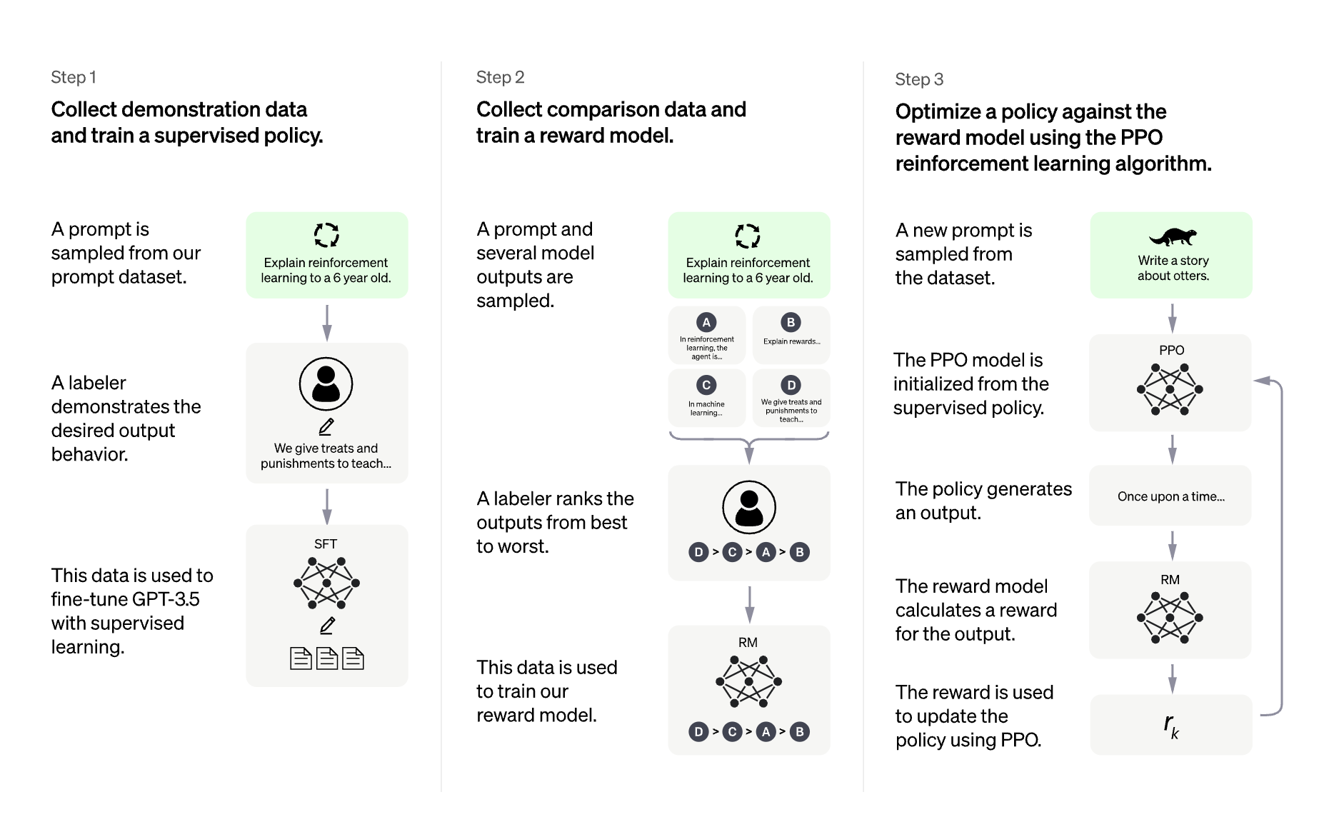
- allows the model to learn from experience and adapt to new situations in real-time.
- It interacts with an environment and receives feedback in the form of rewards or penalties, allowing it
to learn which actions lead to desirable outcomes.
- The goal is to learn a policy that maximizes the expected cumulative reward over a sequence of actions,
given a particular state, while also constraining the magnitude of updates to prevent large deviations.
Red teaming: the system is stress-tested by a curated crowd to ensure it’s able to handle real-world scenarios and make accurate and relevant predictions.

Note: add KL penalty - to the full reward maximisation objective via a reference model, which serves to prevent the model from learning to cheat or exploit the reward model.

PPO (schulman et at., 2017): https://arxiv.org/abs/1707.06347

RL scheme (stiennon et al. 2020) https://arxiv.org/abs/2009.01325

11.28.2. Direct Preference Optimization (DPO)

direct likelihood objective can be optimized without the need for a reward model or the need to perform the potentially fiddly RL based optimisation.

steps:

a supervised fine-tuning (SFT) step
the process of annotating data with preference labels
however the DPO training does away with the task of reward modeling and RL (steps 3 and 4) and directly optimizes the DPO object on preference annotated data. (3. training a reward model on the preference data 4. and the RL optmization step)

links
- https://arxiv.org/abs/2305.18290
- https://huggingface.co/blog/dpo-trl

11.28.3. ChatGPT 3 steps

Collect demonstration data and train a supervised policy.
- pretrained transformer-based model is fine-tuned on this dataset combined with the old dataset, which is
transformed into a dialogue format.
get a model that takes in a pair (prompt, text) and returns a scalar reward which should numerically represent the human preference. RM

links
- https://dida.do/blog/chatgpt-reinforcement-learning
- https://arxiv.org/pdf/2203.02155.pdf

11.28.4. links

RL : PPO course https://huggingface.co/learn/deep-rl-course/unit0/introduction

11.29. Language Server

Usually, the parser builds a concrete syntax tree (CST) before turning it into an abstract syntax tree (AST).

AST - data structure used in computer science to represent the structure of a program or code snippet

allow clone detection
an edit action may result in the addition of a new AST node representing a function.

For example, take a simple expression 2 * (7 + 3):

           CST                    AST
          -----                  -----
          expr                     *
       /   |    \                /   \
  term     *   term             2     +
   |             |                   / \
factor         factor               7   3
   |         /   |    \
   2        (   expr   )
              /  |  \
          term   +  term
            |        |
          factor   factor
            |        |
            7        3

https://supabase.com/blog/postgres-language-server-implementing-parser

11.30. GPT

steps:

first we train a transformer model on a very large amount of data in an unsupervised manner—using language modeling as a training signal
we fine-tune this model on much smaller supervised datasets to help it solve specific tasks.

12. LLM, chat bots, conversational AI, intelligent virtual agents (IVAs)

LLM intro https://www.youtube.com/watch?v=zjkBMFhNj_g

Slides as PDF: https://drive.google.com/file/d/1pxx_ZI7O-Nwl7ZLNk5hI3WzAsTLwvNU7/view?usp=share_link (42MB)
Slides. as Keynote: https://drive.google.com/file/d/1FPUpFMiCkMRKPFjhi9MAhby68MHVqe8u/view?usp=share_link

positively impacted by AI bot solutions as below:

Eliminate wait times: Customers today look for faster response times across all aspects of their daily lives. But, during peak times, agents can become overburdened responding to multiple inbound requests, requiring incoming customer calls or chats to be in a queue. As the queue increases and waiting times prolong, customers might abandon or get frustrated, leading to poor experience and potential business loss.
Reduce Missed Chats or Abandon Rate: Live chat abandon rates can represent missed business opportunities and poor experience. Most of the time, the connection to the live chat agent breaks down, requiring the customer to start from scratch and launch a new chat window. Chatbots operate in an asynchronous mode where customers can start, pause, or continue a conversation hours later without having to start everything from scratch.
Shortens Average Agent Handling Time: A bot can assist an agent by providing them with suggested responses or information and automating the underlying tasks that better support the agent in responding faster. Since the bot can also detect customer intent, it can speed up access to the correct information and automate the live chat interaction. This is key to making agents more productive and resolving customer issues faster.
Increases accuracy and consistency: Although a customer gets through an agent, there are still chances of not obtaining the right or complete information. This can lead to serious consequences for businesses as well as their customers. AI bots alongside virtual agents can often bring the best results, where the former responds to routine requests and automates underlying workflows while the latter can tackle more complex issues with emotional intelligence.
Improves customer experience and retention: The application of AI within customer care centers is not just confined to handling simple customer requests and workflows. They also have the capability to automate complex customer journeys such as customer onboarding, subscription renewals, and claims management, all of which lead to increased sales conversion, higher retention, faster resolution, and more.
Enhances productivity and satisfaction: Chatbots working alongside agents can help automate routine workflows, allowing agents to free up from mundane tasks and focus on areas…

цепочки и деревья команд к LLMs: CoT, ToT, Self-Consistency, ReAct ?

Chain of Thoughts, Tree of Thoughts, ReAct

byte-pair encoding

GPT4 -> AutoGPT -> ChatDev MetaGPT -> AutoGen

12.1. terms

the context length

context window

is a range of tokens the model can consider when generating responses to prompts. GPT-3=2k, GPT-4=32k - cost increase quadratically or at least linear. Measured in count of tokens.

can be fixed or variable size - input have context window and target token position.
during training used to learn, during prediction the context window generates predictions.

(no term)

key-value head see 10.15.6.5

autoregressive

refers to the fact that the model generates its output one step at a time, based on the previous steps.

Self-supervised data

labels or annotations are generated automatically from the data itself.

Supervised Fine-tuning step (SFT)
Reward Modeling step (RM)
Proximal Policy Optimization (PPO) step - 2017 Proximal Policy Optimization Algorithms https://arxiv.org/pdf/1707.06347.pdf

12.2. history

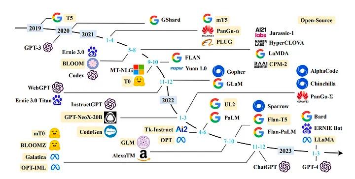
12.3. free chatgpt api

12.4. instruction-following LLMs

Training language models to follow instructions with human feedback https://arxiv.org/abs/2203.02155

12.5. DISADVANTAGES AND PROBLEMS

pop
not deep
not answer close and dont explain topic - it is to logic

12.6. ability to use context from previous interactions to inform their responses to subsequent questions

tech "dialogue context" to maintain a conversation's state
tech "teacher forcing,"
tech "prompt engineering" - does not have memory or knowledge, instead: converstation history is concatenated into a single text prompt, with each message or response separated by a special delimiter.

reinforcement learning used for fine-tuning.

12.7. GigaChat Sber

GigaChat работает на

языковых моделях ruGPT-3 и FRED-TP
нейросетевой ансамбль NeONKA (NEural Omnimodal Network with Knowledge-Awareness)
https://habr.com/ru/companies/sberdevices/articles/730088/
https://habr.com/ru/companies/sberdevices/articles/564440/
https://habr.com/ru/companies/sberbank/articles/730108/

18 миллиардах параметров

картинки uCLIP и Kandinsky 2.1

12.8. GPT - Generative Pre-trained Transformer

12.9. llama2

python-ds#MissingReference

12.9.1. theory

Meta's Llama 1
Llama2 product of an uncommon alliance between Meta and Microsoft,
Llama 2 was trained with 40% more data than its predecessor

LLama1 - based on transformer architecture - 65B trained on 2048 x 80GB RAM GPUs - dataset 1.4T tokens - 21 days

Pre-normalization [GPT-3] - RMSNorm
SwiGLU activation [PALM] - replace the ReLU - for performance
Rotary Embeddings [GPTNeo] - replace absolute embeddings with RoPE at each layer of the nerwork.
optimizer - AdamW with cosing learning rate schedule - final learning rate is 10% of the max lr.
optimizations:
- causal multi-head attention - to reduse memory usage
- reduce amount of activations with checkpointing: replace PyTorch autograd with custom.
- overlap comps between GPUs over the network (due to all_reduce operations)
Context length 2k

Warmup steps are just a few updates with low learning rate before / at the beginning of training. After this warmup, you use the regular learning rate (schedule) to train your model to convergence.

LLama2 - is auto-regressive transformer pretrained on an corpus of self-supervised data, followed by alignment with human preferences via RLHF.

Supervised fine-tuning used an autoregressive loss function with token loss on user prompts zeroed out. (wiki)
Batch size was 64 (wiki)
2T tokens dataset
Context length 4k
Grouped Query Attention (GQA) - main difference from LLama1 - speed up decoder inference (hf.com)
steps:
1. supervised learning (LLama2) - chat backpropageted только ответы, 27540 анотоций, 2 epochs, cosine
learning rate, init. lr=2e-05, w. decay=0.1 batch=64.
1. supervised fine-tuning (LLama-2-chat)
2. Rejection Sampling -> Proximal Policy Optimization PPO (cycle)
3. Human feedback
lateralization logic framework, literalization pathways ?

12.9.2. quantization libraries

HF - Hugging Face pytorch pickle file. file format

GPTQ
- https://huggingface.co/docs/transformers/main_classes/quantization
- https://pypi.org/project/gptq/
- Torch
- 2/3/4/8-bit quantized matrix full-precision vector product CUDA kernel
ggml https://github.com/ggerganov/ggml
bitsandbytes https://pypi.org/project/bitsandbytes/
- Torch ?
Quantization allows PostgresML to fit larger models in less RAM.

comparizaion
https://github.com/ggerganov/llama.cpp/discussions/2424

I've run GPTQ and bitsandbytes NF4 on a T4 GPU and found:

fLlama-7B (2GB shards) nf4 bitsandbytes quantisation:
- PPL: 8.8, GPU Mem: 4.7 GB, 12.2 toks.
Llama-7B-GPTQ-4bit-128:
- PPL: 9.3, GPU Mem: 4.8 GB, 21.4 toks.
fLlama-13B (4GB shards) nf4 bitsandbytes quantisation:
- PPL: 8.0, GPU Mem: 8.2 GB, 7.9 toks.
Llama-13B-GPTQ-4bit-128:
- PPL: 7.8, GPU Mem: 8.5 GB, 15 toks.
I've also run ggml on T4 and got 2.2 toks, so it seems much slower - whether I do 3 or 5bit quantisation.

12.9.3. jailbreak

https://github.com/facebookresearch/llama-recipes

https://simonwillison.net/2023/Mar/11/llama/?ref=thisismeteor.com

12.9.4. gpt vs llama

AI2 Reasoning Challenge (25-shot) - a set of grade-school science questions.

Llama 1 (llama-65b): 57.6
LLama 2 (llama-2-70b-chat-hf): 64.6
GPT-3.5: 85.2
GPT-4: 96.3

HellaSwag (10-shot) - a test of commonsense inference, which is easy for humans (~95%) but challenging for SOTA models.

Llama 1: 84.3
LLama 2: 85.9
GPT-3.5: 85.3
GPT-4: 95.3

MMLU (5-shot) - a test to measure a text model’s multitask accuracy. The test covers 57 tasks including elementary mathematics, US history, computer science, law, and more.

Llama 1: 63.4
LLama 2: 63.9
GPT-3.5: 70.0
GPT-4: 86.4

TruthfulQA (0-shot) - a test to measure a model’s propensity to reproduce falsehoods commonly found online. Note: TruthfulQA in the Harness is actually a minima a 6-shots task, as it is prepended by 6 examples systematically, even when launched using 0 for the number of few-shot examples.

Llama 1: 43.0
LLama 2: 52.8
GPT-3.5: 47.0
GPT-4: 59.0

12.9.5. fine tuning

see 11.28

TRL + PEFT : https://huggingface.co/docs/trl/index
- trl.SFTTrainer (QLoRA) https://www.philschmid.de/instruction-tune-llama-2
- QLoRA steps:
  1. Quantize the pre-trained model to 4 bits and freeze it.
  2. Attach small, trainable adapter layers. (LoRA)
  3. Finetune only the adapter layers while using the frozen quantized model for context.
- Flash Attention - see 12.9.5.1
PEFT
- huggingface/autotrain-advanced
DPO https://huggingface.co/blog/dpo-trl

Original paper:

Flash Attention - accelerates training up to 3x
- https://github.com/Dao-AILab/flash-attention/tree/main
- "FlashAttention: Fast and Memory-Efficient Exact Attention with IO-Awareness" https://arxiv.org/abs/2205.14135
```
python -c "import torch; assert torch.cuda.get_device_capability()[0] >= 8, 'Hardware not supported for Flash Attention'"
```
```
pip install ninja packaging
MAX_JOBS=4 pip install flash-attn --no-build-isolation
```
usage examples:
- https://www.philschmid.de/instruction-tune-llama-2#3-instruction-tune-llama-2-using-trl-and-the-sfttrainer
DPO
- DPO - Direct Preference Optimization
cast the RL-based objective used by existing methods to an objective which can be directly optimized via a simple binary cross-entropy loss which simplifies this process of refining LLMs greatly.

DPO bypasses the reward modeling step and directly optimises the language model on preference data via a key insight

no need need for a reward model.

see 14.7

DPO https://arxiv.org/abs/2305.18290
1. DPO vs PPO
  - PPO - Proximal Policy Optimization
  - https://huggingface.co/blog/dpo-trl
links

12.9.6. stackllama

LlaMa model to answer questions on Stack Exchange

https://huggingface.co/blog/stackllama

12.9.7. distribute

problems:

Data parallelism does not help reduce memory footprint per device
Model parallelism does not scale efficiently beyond a single node due to fine-grained computation and expensive communication. ex. NVIDIA Megatron-LM - at multi-node performance degrades.

links

https://huggingface.co/blog/accelerate-large-models
DeepSpeed
ZeRO - The Zero Redundancy Optimizer - solution for problems - microsoft: "ZeRO-powered data parallelism". see 12.9.7,
- partitioning the model states: parameters, gradients, and optimizer state - (not replicating!)
- dynamic communication schedule during training to share the necessary state across distributed devices to retain the computational granularity and communication volume of data parallelism.
- ZeRO eliminates memory redundancies and makes the full aggregate memory capacity of a cluster available.
Zero https://www.microsoft.com/en-us/research/blog/zero-deepspeed-new-system-optimizations-enable-training-models-with-over-100-billion-parameters/
- https://www.microsoft.com/en-us/research/uploads/prod/2020/02/Turing-Animation.mp4
Turing Natural Language Generation (T-NLG) - Microsoft LModel for NLP task (17B parameters) https://www.microsoft.com/en-us/research/blog/turing-nlg-a-17-billion-parameter-language-model-by-microsoft/

DeepSpeed Chat https://github.com/microsoft/DeepSpeed/tree/master/blogs/deepspeed-chat

https://www.microsoft.com/en-us/research/blog/zero-deepspeed-new-system-optimizations-enable-training-models-with-over-100-billion-parameters/
1. TODO Mixture of Experts (MoE)
  DeepSpeed v0.5 introduces new support
  
  DeepSpeed MoE supports five different forms of parallelism:
  - E Expert Scales the model size by increasing the number of experts
  - E + D Expert + Data Accelerates training throughput by scaling to multiple data parallel groups
  - E + Z Expert + ZeRO-powered data Partitions the nonexpert parameters to support larger base models
  - E + D + M Expert + Data + Model Supports massive hidden sizes and even larger base models than E+Z
  - E + D + Z Expert + Data + ZeRO-powered data Supports massive hidden sizes and even larger base models than E+Z
  - E + Z-Off + M Expert + ZeRO-Offload + Model Leverages both GPU and CPU memory for large MoE models on limited # of GPUs
  Random token selection addresses the limitation of biased selection problem in MoE model training. https://www.deepspeed.ai/tutorials/mixture-of-experts/
TODO torchx
Not all available out-of-the-box.
- Model Parallel
- DDP
https://pytorch.org/torchx/main/components/overview.html

12.9.8. schema trl+deepspeed

SFTTrainer: A light and friendly wrapper around transformers Trainer to easily fine-tune language models or adapters on a custom dataset.

trl is a wraper around huggingface/transformers

12.9.9. wiki at work

Интерфейс к клиенту, что он нам дает?

SFT - вопрос, ответ?

PPO - human-provided rankings of multiple answers to the same query?

DPO - ?
Термины

    LLaMa2 Chat - LLaMa2 модель прошедшая SFT и PPO, веса поставляются как отдельная модель, на равне с LLaMa2.
    Proximal Policy Optimization (PPO)
    Direct Preference Optimization (DPO)
    offloading - разгрузка GPU и перенос вычислений и памяти на CPU.
    Automatic Mixed Precision (AMP) - Автоматическая конвертация параметров в float16 для ускорения. Some ops, like linear layers and convolutions, are much faster in float16 or bfloat16. (PyTorch + Nvidia)
    Automatic loss scaling (ALS) - техника используемая при mixed precision для улучшения стабильности и точности. (DeepSpeed + Nvidia)
    Distributed Data Parallel (DDP) - на каждом GPU/машинам хранится копия параметров и states. (PyTorch)
    Fully Sharded Data Parallel (FSDP) - разделение параметров и states по GPU/машинам и обеспечение возможности offload в CPU. (PyTorch)
    Gradient Clipping -


Дообучение

Этапы дообучения (RLHF):

    supervised fine-tuning (SFT) - в llama2 chat backpropageted только ответы, 27540 анотоций, 2 epochs, cosine learning rate, init. lr=2e-05, w. decay=0.1 batch=64.
    PPO (классическая) или DPO (новая) дообучение. PPO - обучается ranking model, которая затем используется для дообучения, DPO - без ranking model.



Библиотеки:

    huggingface/autotrain-advanced with peft (sft training)
    huggingface/transformers - может использовать: DeepSpeed
    huggingface/trl - может использовать: transformers, PEFT, accelerate
    huggingface/peft - Parameter-Efficient Fine-Tuning (PEFT) - State-of-the-Art PEFT techniques achieve performance comparable to that of full fine-tuning.
    huggingface/accelerate - распределенное обучение, может использовать: DeepSpeed, Megatron-LM
    DeepSpeed - Pipeline-parallelism (kind of model-parallelism), Tensor-parallelism

Библиотеки (к сведению):

    PyTorch Lightening - высокоуровневый интерфейс к PyTorch, поддерживает распределенное обучение: DDP, FSDP, DeepSpeed

Ссылки по приоритету информативность+понятность:

    https://en.wikipedia.org/wiki/LLaMA
    https://huggingface.co/docs/transformers/model_doc/llama2
    LLama 1 (Touvron et al. 2023) https://arxiv.org/abs/2302.13971
    LLama 2 https://arxiv.org/abs/2307.09288
    official inference code https://github.com/facebookresearch/llama
    models https://huggingface.co/models?search=llama2
    Code LLama https://arxiv.org/abs/2308.12950

Трансформер

    https://papers.nips.cc/paper/7181-attention-is-all-you-need.pdf
    https://machinelearningmastery.com/the-transformer-model/
    Improving Language Understanding by Generative Pre-Training https://s3-us-west-2.amazonaws.com/openai-assets/research-covers/language-unsupervised/language_understanding_paper.pdf
    Multi Query Attention (MQA) - используется LLaMa2 для ускорения https://arxiv.org/pdf/2305.13245.pdf
    https://lilianweng.github.io/posts/2023-01-27-the-transformer-family-v2/

Дообучение

1. https://huggingface.co/blog/dpo-trl

2. trl + accelerate https://huggingface.co/blog/trl-peft
Like
Be the first to like this

12.9.10. links

doc First llama (Touvron et al. 2023) https://arxiv.org/abs/2302.13971
llama2 https://arxiv.org/abs/2307.09288
- file:///home/ff/Downloads/2307.09288.pdf
- ? code llama2 https://arxiv.org/abs/2308.12950
? https://arxiv.org/pdf/2305.13245.pdf
- file:///home/ff2/Downloads/2305.13245.pdf
code llama https://arxiv.org/abs/2308.12950
huggungface model description https://huggingface.co/docs/transformers/model_doc/llama2
official inference code https://github.com/facebookresearch/llama
models https://huggingface.co/models?search=llama2
doc https://huggingface.co/docs/transformers/main/model_doc/llama2
doc https://ai.meta.com/research/publications/llama-2-open-foundation-and-fine-tuned-chat-models/?_fb_noscript=1
- https://scontent-iev1-1.xx.fbcdn.net/v/t39.2365-6/10000000_662098952474184_2584067087619170692_n.pdf?_nc_cat=105&ccb=1-7&_nc_sid=3c67a6&_nc_ohc=04ReMOti9ikAX9WxYJw&_nc_ht=scontent-iev1-1.xx&oh=00_AfCzbf3jU5lAs6PLGJH0eFZXj_uaSXnKUDFxzgTd2Y-iBw&oe=64E3F9BF
- /home/ff/Downloads/10000000_662098952474184_2584067087619170692_n.pdf
sub models https://www.reddit.com/r/LocalLLaMA/wiki/models/
download https://easywithai.com/resources/llama-2/
Source – HF – GPTQ – ggml - file formats, not equal to original.

12.10. frameworks to control control LLM

12.11. size optimization

NVIDIA bfloat16 keeps the full exponential range of float32, but gives up a 2/3rs of the precision

Format	Significand	Exponent
bfloat16	8 bits	8 bits
float16	11 bits	5 bits
float32	24 bits	8 bits

12.12. distribute training - choose framework

model parallelism

torch.distributed.rpc - This package allows you to perform a model-parallelism strategy. It is very efficient if your model is large and does not fit in a single GPU.
DeepSpeed - model-parallelism on PyTorch https://github.com/microsoft/DeepSpeed
Mesh TensorFlow - model-parallelism on Tensorflow

Asychronous Data-parallelism

parameter server strategy in Tensorflow and Torch
torch.nn.DistributedDataParallel

Pipeline Parallelism https://people.eecs.berkeley.edu/~matei/papers/2019/sosp_pipedream.pdf

DeepSpeed
PyTorch TODO: https://pytorch.org/tutorials/intermediate/pipeline_tutorial.html

Tensor Parallelism: Model parallelism and Pipeline parallelism split model vertically to slices from input to output. Tensor parallelism split horizontally - every tensor.

Mixture-of-Experts(MoE) -

TensorFlowOnSpark - https://github.com/yahoo/TensorFlowOnSpark

huggingface/accelerate support

DeepSpeed - Current integration doesn’t support Pipeline Parallelism of DeepSpeed, doesn’t support multiple models
Megatron-LM

BigDL Intel for Apache Spark - ?

Horovod Uber - data parallelism only

Ray - data parallelism, Model parallelism

Megatron-LM Nvidia (used in NeMo Megatron) - tensor, pipeline and sequence based model parallelism for pre-training transformer based Language Models - Transformers

Nvidia and Apache License 2.0 for Facebook, huggingface and Google Research code
https://github.com/NVIDIA/Megatron-LM
Model parallelism https://arxiv.org/abs/1909.08053
GPU Clusters https://people.eecs.berkeley.edu/~matei/papers/2021/sc_megatron_lm.pdf
https://huggingface.co/docs/accelerate/usage_guides/megatron_lm

DeepSpeed Microsoft - empowers ChatGPT-like model training

Apache License 2.0
deepspeed.ai
https://github.com/microsoft/DeepSpeed

ColossalAI - Data Parallelism, Tensor Parallelism - single machine?

Yandex - decetralized - LLama, Falcon https://github.com/bigscience-workshop/petals

12.12.1. wiki work

Термины

microbatches - используется в PyTorch Pipeline Parallelism как разбиение батчей, для обеспечения data parallelism. В TF Mirrored Strategy называется "batch per replica".

Парадигмы

Model parallelism

Не используется в отдельности без pipeline parallelism, так как в одинмомент времени задействована только 1 машина.
torch.distributed.rpc - This package allows you to perform a model-parallelism strategy. It is very efficient if your model is large and does not fit in a single GPU.
- https://pytorch.org/tutorials/intermediate/dist_pipeline_parallel_tutorial.html
- ResNet50 https://github.com/pytorch/examples/blob/main/distributed/rpc/pipeline/main.py
DeepSpeed - model-parallelism on PyTorch https://github.com/microsoft/DeepSpeed
Mesh TensorFlow - model-parallelism on Tensorflow
Pytorch TorchX - model-parallelism, DDP, may not work out-of-the-box. Универсальный запускатель задач, использует distributed.elastic. Fault-tolerance ориентирован.

Asychronous Data-parallelism

parameter server strategy in Tensorflow and Torch
torch.nn.DistributedDataParallel

Pipeline Parallelism

https://people.eecs.berkeley.edu/~matei/papers/2019/sosp_pipedream.pdf
DeepSpeed
PyTorch - torch.distributed.pipeline - Pipe only supports intra-node pipelining currently!
- Transformers https://pytorch.org/tutorials/intermediate/pipeline_tutorial.html
- https://pytorch.org/docs/stable/pipeline.html
- 2020 "torchgpipe" https://arxiv.org/abs/2004.09910
- 2019 https://arxiv.org/abs/1811.06965

Tensor Parallelism - в отличии от pipeline, model parallelism - горизонтальный, разделяет каждый тензон. Используется для Inference?

PyTorch - experimental! https://pytorch.org/docs/stable/distributed.tensor.parallel.html

PyTorch - native

DistributedDataParallel (DDP) + Model parallelism - необходимо вручную разбить модель на части.
- https://pytorch.org/tutorials/intermediate/ddp_tutorial.html
DDP + torch.distributed.rpc - hybrid parallelism - часть модели разделяется между воркерами, другая часть дублируется, вручную.
- https://pytorch.org/tutorials/advanced/rpc_ddp_tutorial.html
FSDP - (как расширенный DDP) можно автоматически разделить слои по машинам по размеру или другим признакам. 4x larder models compared to DDP and 20x larger with activation checkpointing and activation offloading.

Список высокоуровневых библиотек

Huggingface/accelerate

DeepSpeed в режиме Pipeline Parallelism не поддерживается в huggingspace сейчас https://huggingface.co/docs/accelerate/usage_guides/deepspeed#few-caveats-to-be-aware-of
Megatron-LM
TRL - просто обертка для Transformers и Accelerate

FairScale by Meta, facebook. FSDP oriented. автоматический mixed precision и шардирование данных, Масштабированная оптимизация

Megatron-LM by Nvidia (used in NeMo Megatron) - "pipeline model parallelism"? model-parallel (tensor, sequence, and pipeline) for Transformers

https://github.com/NVIDIA/Megatron-LM
Model parallelism https://arxiv.org/abs/1909.08053
GPU Clusters https://people.eecs.berkeley.edu/~matei/papers/2021/sc_megatron_lm.pdf
https://huggingface.co/docs/accelerate/usage_guides/megatron_lm

DeepSpeed by Microsoft - pipeline parallelism

Apache License 2.0
deepspeed.ai
https://github.com/microsoft/DeepSpeed
https://www.microsoft.com/en-us/research/uploads/prod/2020/02/Turing-Animation.mp4

PyTorch Lightning - Apache 2.0

TensorFlowOnSpark - https://github.com/yahoo/TensorFlowOnSpark

BigDL Intel for Apache Spark - ?

Horovod Uber - data parallelism only

Ray - data parallelism, Model parallelism

ColossalAI - Data Parallelism, Tensor Parallelism - single machine?

Ссылки

Лучшие статьи о парадигмах:

https://huggingface.co/docs/transformers/v4.17.0/en/parallelism
https://lilianweng.github.io/posts/2021-09-25-train-large/
comparision of distributed ml systems https://arxiv.org/pdf/1909.02061.pdf

Ссылки

Like Be the first to like this

12.12.2. links

12.13. TODO bots

Pyrogram или AIOGram

12.14. Fine-tuning

https://magazine.sebastianraschka.com/p/finetuning-llms-with-adapters

Feature-based approach - frozen all transformer + output embedding - train only classifier.
- pre-training real-valued embeddings vectors.
Finetuning 1 - keep frozen all except 1 or more fully connected layers - PEFT
Finetuning 2 - update all layers
Adapter mudules - bottleneck architecture - PEFT

proximal policy optimization PPO - online policy gradient method

steps of training:

Pretraining on unlabeled text corpus - unsupervised pretraining
finetune all model or PEFT (with frozen layers and new ones)

12.14.1. Parameter-Efficient Finetuning techniques (PEFT)

finetune LLM while require the training of only a small number of parameters

subset of the existing model parameters - or set of newly added parameters
does the method aim to minimize memory footprint or only storage efficiency

types:

additive - augmenting the existing pre-trained model with extra parameters or layers and training only the newly added
- adapters - add additional parameters to each transformer block.
- prompt tuning or modifications - hard or soft or prefix tuning (as LLaMa adapter) - appends a tensor to
the embedded inputs of a pretrained LLM
- soft prompts - consists of a task description accompanied by a few in-context examples
selective - fine-tuning only selected layers/biases/rows
reparametrization-based (kind of additive) - leverage low-rank representations to minim the number of trainable parameters. Low-rank subspace finetuning. Part of the model's input embeddings is fine-tuned via gradient descent.
- Fastfood transform to reparametrize the update to NN params.
- LoRa - simple low-rank matrix decomposition(or Kronecker product decomposition) to parametrize the weight
update

In case of Adam, for every byte of trainable parameter, one extra byte is needed for its gradient, and two more bytes are needed to store the optimizer state: the first and second moments of the gradient.

= 3x
training a model re quires 12-20 times more GPU memory than the model weights

Adapters - additive type

2019 https://arxiv.org/pdf/1902.00751.pdf Parameter-Efficient Transfer Learning for NLP

fully connected layers of the adapters are usually relatively small and have a bottleneck structure similar to autoencoders.

ex. input 1024, first layer 24 -> 1,024 x 24 + 24 x 1,024 = 49,152 weight parameters.

1,024 x 1024 = 1,048,576 # if first layers would have 1024 - it would be too many parameters

Performance compatible with full fine-tuning by tuning less than 4% of the totam model params.

def transformer_block_with_adapter(x):
    residual = x
    x = self_attention(x)
    x = AdapterLayers(x) # adpater
    x = LayerNorm(x + residual)
    residual = x
    x = FullyConnectedLayer(x)
    x = AdapterLayers(x) # adpater
    x = LayerNorm(x + residual)
    return x

def AdapterLayers(x):
    residual = x
    x = SmallFullyConnectedLayer(x) # to a low-dimensional representation
    x = ReLU(x) # NonlinearActivation
    x = FullyConnectedLayer(x) + residual #  back into the input dimension
    return x

LoRA - Low rank adaptation (LoRA) - reparameterization type
- https://arxiv.org/pdf/2106.09685.pdf LORA: LOW-RANK ADAPTATION OF LARGE LANGUAGE MODELS
- article https://habr.com/ru/articles/747534/
LoRA - freezes the pretrained model weights and injects trainable rank decomposition matrices into each layer of the Transformer architecture, greatly reducing the number of trainable parameters for downstream tasks.
TODO BitFit - selective type
links
https://arxiv.org/abs/2303.15647 Comparision of PEFT methods
- Bitfit: Simple parameter-efficient fine-tuning for transformer-based masked language-models. ArXiv, abs/2106.10199.
- Lora: Low-rank adaptation of large language models. ArXiv, abs/2106.09685
- Rabeeh Karimi Mahabadi, James Henderson, and
Sebastian Ruder. 2021. Compacter: Efficient low-rank hypercomplex adapter layers. In Ad- vances in Neural Information Processing Sys- tems, volume 34, pages 1022–1035. Curran As- sociates, Inc

12.14.2. multi-task learning

Sharing network parameters (weights) across tasks (in lower layers) exploits task regularities, yielding improved performance.

A single model to solve all problems.

12.15. pipeline

12.15.1. types:

Advantages:
- simple
- modular
- Efficient
compose your own
Off-the-shelf
legacy class
LCEL
- streaming
- Async (and sync) support
- Optimized parallel execution
- Integrated with LangSmith and LangServe

12.15.2. use cases

QA over structured data: Qustion -> SQL Query -> Query result -> additional context -> answer
Extraction: Unstructured Text + JSON Schema ➞ Compiled JSON
Summarization: MOAR text ➞ LESS text
Synthetic data generation: JSON Schema ➞ [Unstructured Text, Unstructured Text, Unstructured Text, Unstructured Text …]
Agents: let LLM takes actions

12.15.3. RAG-пайплайн

https://arxiv.org/abs/2005.11401 2020 Retrieval-Augmented Generation for Knowledge-Intensive NLP Tasks
rag https://towardsdatascience.com/rag-vs-finetuning-which-is-the-best-tool-to-boost-your-llm-application-94654b1eaba7
https://towardsdatascience.com/retrieval-augmented-generation-rag-from-theory-to-langchain-implementation-4e9bd5f6a4f2

RAG - It combines a retriever system, which fetches relevant document snippets from a large corpus, and an LLM, which produces answers using the information from those snippets

LLM gets queru + found context to finetune.

docs = retriver.get_relevant_documents(question)

context = "\n\n".join(doc.page_content for doc in docs)

prompt_val = prompt.invoke({"context": context, "question": questions})

result = llm(prompt_val.to_message())

12.16. tools

Weaviate: vector database (https://weaviate.io/)
LangChain: pipeline orchestration

12.17. LangChain

Tools, Models, Example selectors, Text splitters, Promts, Output Parsers, Vector Stores

pros:

Python (also JS/TS) framework
Building blocks
Swappable components
Examples
From PoC to Production
Speed of improvement

Text Splitters: 5 levels of text splitting:

Characters / Tokens
Recursive Character
Document structure
Semantic Chunker
Agent-like Splitting

12.18. Most Used Vectorstores

Chroma
FAISS
Pinecone
drant
docarray
weaviate
PostrgreSQL
supabase
neo4j
redis
Azure Cognitive Search
Astra DB

12.19. LLM Providers

OpenAI
A? OpenAI - microsoft?
Anthrop\c
HuggingFace
Vertex AI
fireworks.ai
ollama
amazon Bedrock

2 OSS Model providers

Huggingface
fireworks.ai
ollama
LLAMA.CPP
replicate
GPT4ALL
together.ai
anyscale

12.20. Promt Engineering vs Train Foundation Models vs Adapters

Promt Engineering

pros
- Do not require GPUs or vast amount of data
- Very practical for fast, iterative problem solving
cons: Limited capabilities, highly dependent on foundation model capabilities.

Train Foundation Models

pros: Very good bragging material
cons:
- Require amounts of data and GPUs - inaccessible to most
- Very risky: no guarantee that it will solve the actual problem you may want it for

Adapters

12.21. TODO Named tensor notation.

ArXiv, abs/2102.13196
ArXiv 2303.15647

12.22. links

https://papers.nips.cc/paper/7181-attention-is-all-you-need.pdf

13. Adversarial machine learning

GAN 10.20

Attacks

evasion attacks: уклонение. spam, biometric verification systems.
data poisoning attacks: contaminating the training dataset ??????
Byzantine attacks: .
model extraction

13.1. linear classifiers - spam - evasion attacks

14. huggingface.co

https://github.com/huggingface

goal of democratising AI, collection of models and datasets

14.1. pip packages

pypi.org/project/huggingface-hub/
- The Hugging Face Hub is a platform with over 90K models, 14K datasets, and 12K demos
- use Cloudfront (a CDN) to geo-replicate downloads
- Inference API - require API_TOKEN
Repository class - wrapper around the git command
HfApi client - HTTP requests

14.2. main projects

huggingface.co/transformers

Transformers is our natural language processing library and our hub is now open to all ML models, with support from libraries like Flair, Asteroid, ESPnet, Pyannote, and more to come.

Inference API

A service-level agreement (SLA) is a contract between two companies or internal teams.
Use the Inference API shared infrastructure for free, or switch to dedicated Inference Endpoints for production
plans:
- free - up to 1M input characters /mo, up to 2 hours of audio. Shared resources, no auto-scaling, standard latency
- Enterprise support for Inference Endpoints. Custom pricing based on volume commit. Starts at $2k/mo, annual contracts
API that allow the programmer to engage with the library at various levels of abstraction.
pipeline, which handles everything for us, namely converting raw text into a set of predictions from a fine-tuned model.

huggingface.co/models -

Accelerate - is a library that enables the same PyTorch code to be run across any distributed configuration

14.3. reduce inference

14.3.1. quantization

Discrete quantization: Going beyond 16-bit down to 8 or 4 bits

quantize transformers model from scratch: ~5 min on a Google colab for facebook/opt-350m model

load models that has been already quantized by other users

links
- https://huggingface.co/docs/transformers/main_classes/quantization
- https://arxiv.org/abs/2210.17323

14.3.2. TODO pruning

removing weights, filters, neurons or even layers that are not necessary after learning.

model distilation: original network teach another shallow network.

magnitude pruning - unstructured pruning method

links
- model distillation [Hinton et al., 2015] https://doi.org/10.1126/science.1127647
- Knowledge Distillation [Gou et al., 2020] https://arxiv.org/abs/2006.05525
- https://pytorch.org/tutorials/intermediate/pruning_tutorial.html

14.4. transformers

14.4.1. base

pipeline - easiest and fastest way to use a pretrained model

AutoClass - automatically infer and load the correct architecture from a given checkpoint

work under hood
There is one class of AutoModel for each task, and for each backend (PyTorch, TensorFlow, or Flax).

AutoModel

for text: AutoModelForSequenceClassification or TFAutoModelForSequenceClassification
TFAutoModel for TF

transformers.Trainer

supports distributed training and mixed precision,

import torch
# - pipeline:
from transformers import pipeline
speech_recognizer = pipeline("automatic-speech-recognition", model="facebook/wav2vec2-base-960h")

# - AutoModel
from transformers import AutoModelForSequenceClassification
model_name = "nlptown/bert-base-multilingual-uncased-sentiment"
pt_model = AutoModelForSequenceClassification.from_pretrained(model_name)
# - ?
from transformers import AutoTokenizer
model_name = "nlptown/bert-base-multilingual-uncased-sentiment"
tokenizer = AutoTokenizer.from_pretrained(model_name)
pt_batch = tokenizer(
    ["We are very happy to show you the 🤗 Transformers library.", "We hope you don't hate it."],
    padding=True,
    truncation=True,
    max_length=512,
    return_tensors="pt",
)
pt_outputs = pt_model(**pt_batch) # preprocessed batch of inputs
pt_predictions = nn.functional.softmax(pt_outputs.logits, dim=-1) # probobilitices for classes

# - Train
model = AutoModelForSequenceClassification.from_pretrained(model_name)
from transformers import TrainingArguments, Trainer
training_args = TrainingArguments(output_dir="test_trainer")  # where to save the checkpoints from your training:
trainer = Trainer(
    model=model,
    args=training_args,
    train_dataset=small_train_dataset,
    eval_dataset=small_eval_dataset,
    compute_metrics=compute_metrics,
)
trainer.train()


# - Fine-tuning:

14.4.2. scipts

https://huggingface.co/docs/transformers/run_scripts

https://github.com/huggingface/transformers/examples/pytorch/summarization/run_summarization.py

TensorFlow scripts utilize a MirroredStrategy for distributed training

Accelerate:

pip install git+https://github.com/huggingface/accelerate
$ accelerate config
$ accelerate test

# - single
python examples/pytorch/summarization/run_summarization.py \
    --model_name_or_path t5-small \
    --do_train \
    --do_eval \
    --dataset_name cnn_dailymail \
    --dataset_config "3.0.0" \
    --source_prefix "summarize: " \
    --output_dir /tmp/tst-summarization \
    --per_device_train_batch_size=4 \
    --per_device_eval_batch_size=4 \
    --overwrite_output_dir \
    --predict_with_generate

# - distributed
python -m torch.distributed.launch \
    --nproc_per_node 8 pytorch/summarization/run_summarization.py \
    --fp16 \
    --model_name_or_path t5-small \
    --do_train \
    --do_eval \
    --dataset_name cnn_dailymail \
    --dataset_config "3.0.0" \
    --source_prefix "summarize: " \
    --output_dir /tmp/tst-summarization \
    --per_device_train_batch_size=4 \
    --per_device_eval_batch_size=4 \
    --overwrite_output_dir \
    --predict_with_generate

# - acelerate
accelerate launch run_summarization_no_trainer.py \
    --model_name_or_path t5-small \
    --dataset_name cnn_dailymail \
    --dataset_config "3.0.0" \
    --source_prefix "summarize: " \
    --output_dir ~/tmp/tst-summarization

14.5. accelerate - DISTRIBUTED

accelerator.prepare(
replace loss.backward() with accelerator.backward(loss)

The "correct" way to launch multi-node training is running $ accelerate launch my_script.py –accelerate_config.yml on each machine

14.5.1. hello world

from accelerate import Accelerator

accelerator = Accelerator()

train_dataloader, eval_dataloader, model, optimizer = accelerator.prepare(
    train_dataloader, eval_dataloader, model, optimizer
)

for epoch in range(num_epochs):
    for batch in train_dataloader:
        outputs = model(**batch)
        loss = outputs.loss
        accelerator.backward(loss)

        optimizer.step()
        lr_scheduler.step()
        optimizer.zero_grad()
        progress_bar.update(1)
# -- replace the typical loss.backward() in your training loop with 🤗 Accelerate’s backwardmethod:

14.5.2. links

14.6. PEFT - DISTRIBUTED

Parameter-Efficient Fine Tuning methods freeze the pretrained model parameters during fine-tuning and add a small number of trainable parameters (the adapters) on top of it

very memory-efficient with lower compute usage while producing results comparable to a fully fine-tuned model.
leveraging DeepSpeed and Big Model Inference

severl Methods

integrated with Accelerate for large scale models leveraging DeepSpeed and Accelerate's Big Model Inferencing capabilities.

14.6.1. links

14.7. TRL

Transformer Reinforcement Learning

train transformer language models and stable diffusion models with Reinforcement Learning, from the Supervised

Fine-tuning step (SFT)
Reward Modeling step (RM)
Proximal Policy Optimization (PPO)

see 11.28

also to fine-tune a model to

generate positive movie reviews, https://huggingface.co/docs/trl/sentiment_tuning
do controlled generation https://github.com/lvwerra/trl/blob/main/examples/sentiment/notebooks/gpt2-sentiment-control.ipynb
make the model less toxic. https://huggingface.co/docs/trl/detoxifying_a_lm

Allow distributed - leverage accelerate from the Hugging Face ecosystem to make this possible

14.7.1. links

14.8. Spaces

showcase your work in the form of self contained ML demo apps

you can choose any licence type

SDK. At the time of writing you can pick from two Python based frameworks for hosting apps: Gradio or Streamlit. Alternatively you can just use custom HTML.

14.9. cache and offline mode

14.9.1. transformers

~/.cache/huggingface/hub https://huggingface.co/docs/transformers/installation?highlight=transformers_cache#cache-setup

offline

env: TRANSFORMERS_OFFLINE=1 HF_DATASETS_OFFLINE=1.

HF_DATASETS_OFFLINE=1 TRANSFORMERS_OFFLINE=1 python examples/pytorch/translation/run_translation.py --model_name_or_path t5-small --dataset_name wmt16 --dataset_config ro-en ...

save_pretrainde and from_pretrained
- default with download:

AutoTokenizer.from_pretrained("bigscience/T0_3B") ; AutoModelForSeq2SeqLM.from_pretrained("bigscience/T0_3B")

save:

.save_pretrained("./your/path/bigscience_t0") ; .save_pretrained("./your/path/bigscience_t0")

offline use:

.from_pretrained("./your/path/bigscience_t0") ; .from_pretrained("./your/path/bigscience_t0")

huggingface_hub
1. python -m pip install huggingface_hub
2. from huggingface_hub import hf_hub_download
3. hf_hub_download(repo_id="bigscience/T0_3B", filename="config.json", cache_dir="./your/path/bigscience_t0")

14.10. Main concepts

Model classes

PyTorch models (torch.nn.Module
Keras models (tf.keras.Model)
JAX/Flax models (flax.linen.Module)

Configuration classes - store the hyperparameters required to build a model (such as the number of layers and hidden size).

pretrained model has Configuration class inside

Preprocessing classes - convert the raw data into a format accepted by the model.

tokenizer - strings
Image processors - vision inputs
feature extractors - audio inputs
processor - multimodal inputs

14.11. problems:

requests.exceptions.SSLError: HTTPSConnectioPool(host='huggingface.co', port=443): Max retries exceeded with url

14.12. pip install gradio_client

https://github.com/gradio-app/gradio

import sys
import time
from gradio_client import Client

client = Client("ysharma/Explore_llamav2_with_TGI", hf_token="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")
# client = Client("abidlabs/my-private-space", hf_token="...")
result = client.predict(
                                "Howdy!",       # str in 'parameter_6' Textbox component
                                api_name="/chat"
)
job = client.submit(str(sys.argv[1:]), api_name="/chat")
while not job.done():
    time.sleep(0.5)
    print(job.outputs()[-1])
# info about api:
client.view_api(return_format="dict")
# not working:
result = client.predict("How are you, I am fine, can you cum?")
print(result)

upload_url = self.src, utils.UPLOAD_URL)
reset_url = self.src, utils.RESET_URL)
api_url = self.src, utils.API_URL
api_info_url = self.src, API_INFO_URL or utils.RAW_API_INFO_URL

14.13. sci-libs/huggingface_hub

pip install huggingface_hub[inference] An async version of the client is also provided, based on asyncio and aiohttp. You can either install aiohttp directly or use the [inference].

pip install huggingface_hub[inference]
export HUGGINGFACE_TOKEN=?? # not password
huggingface-cli login --token $HUGGINGFACE_TOKEN
# Your token has been saved to /root/.cache/huggingface/token

text-generation-inference backend (TGI) - ? https://github.com/huggingface/text-generation-inference.

transformers + api-inference solution is still in use. - ?

InferenceClient

from huggingface_hub import InferenceClient
client = InferenceClient()
image = client.text_to_image("An astronaut riding a horse on the moon.")
image.save("astronaut.png")

InferenceClient my

from huggingface_hub import InferenceClient
client = InferenceClient(model="upstage/llama-30b-instruct-2048", token=True, timeout=25, headers={}, cookies={})
o = client.text_generation(prompt="An astronaut riding a horse on the moon?")

InferenceClient Async my

from huggingface_hub import AsyncInferenceClient
client = AsyncInferenceClient(model="upstage/llama-30b-instruct-2048", token=True, timeout=25, headers={}, cookies={})
o = await client.text_generation(prompt="An astronaut riding a horse on the moon?")

links

14.13.1. links

free inference with spaces:

14.14. autotrain

workflow

Task
- Vision
  - Image Classification - is the task of classifying images into an arbitrary number of groups.
- Text
  - Text Classification (Binary) - is the task of classifying texts into two distinct groups.
  - Text Classification (Multi-class) - is the task of classifying texts into an arbitrary number of groups, each sample belonging to only one group
  - Token Classification - is the task of classifying certain entities (persons, locations, nouns, verbs…) present in a text into a given number of groups.
  - Question Answering (Extractive) - is the task of retrieving the answer to a question from a context
  - Translation - is the task of translating a text from a language to another
  - Summarization - is the task of summarizing a document or an article into a shorter text.
  - Text Regression - is the task of attributing a score to a text.
- Tabular
  - Tabular Data Classification (Binary) is the task of classifying tabular data into an arbitrary number of groups, each sample belonging to only one group.
  - Tabular Data Classification (Multi-class) is the task of classifying tabular data into an arbitrary number of groups, and each sample can belong to several groups.
  - Tabular Data Regression is the task of attributing a score to tabular data.
Model choice (Automatic, Manual)
Data
- Method 1: Pre-arranged folders
- Method 2: CSV/JSONL with associated images

14.15. links

15. OLD deploy tf keras

16. deeppavlov lections

Seminar 1. Part 1 https://www.youtube.com/watch?v=3nKhzlfaOTE
- Conversional AI
- 2015 messengers > social networks
- request -> Modular Dialog system - > NLU (domain detection, intent detection, Entities detection) -> Dialogue manager (dialogue state, policy) -> Natural Language Generator (Generative models, Templates) -> answer
- Encoder LSTMs -> attention -> Decoder LSTMs -> softmax
- Embedding or Encoder -> memory ->Attention (current input and state) ->Decoder or Action generator
- Нейросеть работает быстрее правил
- Language models на огромной выборке данных и использовать для решения NLP задач
  - BERT
  - OpenAI
  - ESIM+ELMO
  - ESIM
  - LSTM+GloVe
  - FastText
- Алиса - Yandex, AliMe Assis - wechat ( если не может дать ответ, переключает на оператора), Xiaolce - Microsoft in China, Google Assistent, Amazon - Aleksa
  - Chit-chat - Seq2seq -> seq2seq with conv context ->knowledge-grounded seq2seq
  - Task-oriented - Single-domain sytem-initiative -> Multi-domain, contextual, multi-initiative -> End-to-end learning, massively multi-domain
- Hype cycle of Gartner - Hype Cycle for Emerging Technologies, 2018
- Значительную часть интеллекта в Алексу добляют третьи стороны
- Minsky's 'Society of mind' - мозг - общество когнитивных агентов
- МФТИ(исследования) -> DeepPavlov <- DeepReplay (сбербанк)(платформенные решения в виле сервисов) ( потребности рынка)
Seminar 1. Part 2. https://www.youtube.com/watch?v=U_1xdGUQZ5o
Seminar 1. Part 3. skipgram cbow https://www.youtube.com/watch?v=juDdkybtTv0
- есть какой-то стендфордский курс
- простейшая модель классификации: x - вектор, U - matrix p(y(x) = k) = softmax(U*x)=> Pk = exp(Uxk)/∑k(exp(Ux))
Stanford Lecture 4: Word Window Classification and Neural Networks https://www.youtube.com/watch?v=uc2_iwVqrRI
Seminar 2. Part 1 https://www.youtube.com/watch?v=92Ctk9OzlDg
- слова в word2vec без дополнительного обучения плохо работают для sentiment
Seminar 2. Part 2 https://www.youtube.com/watch?v=1zv1IJAS9r4
- elu лучше, но медленее считается
- градиентный спуск

17. passport

rec:

colour:

rectangle:

https://stackoverflow.com/questions/26583649/opencv-c-rectangle-detection-which-has-irregular-side
OpenCV shape detection https://www.pyimagesearch.com/2016/02/08/opencv-shape-detection/
https://robotclass.ru/tutorials/opencv-detect-rectangle-angle/
https://towardsdatascience.com/object-detection-with-neural-networks-a4e2c46b4491
https://github.com/jrieke/shape-detection
MRZ https://web.archive.org/web/20140801191250/http://www.fms.gov.ru/upload/iblock/fe3/prikaz_mchz279.pdf
https://github.com/Shreeshrii/tessdata_ocrb
Машиночитаемая запись МЧЗ
двух строк по 44 символа
Шрифт OCR-B type 1 (Стандарт ИСО 1073/II).
верхняя строка 6-44 модернизированный клер
10, 20, 28, 43, 44 нижней строки МЧЗ содержат контрольные цифры.
top
- 1-2 PN Passport National - Тип документа
- 3-5 RUS - код ИКАО
- 6-44 BAQRAMOV<<AMIR<IL9GAM<<0GLY<<<<<<<<<<<< - БАЙРАМОВ \n АМИР \n ИЛЬГАМ - ОГЛЫ
  - дефис = '<' - знак заполнитель
  - имя сокращается на букве, которая является 42 знаком строки, знака-заполнителя вносится первая буква отчества.
  - фамилия сокращается на букве, которая является 39 знаком строки, после двух знаков-заполнителей последовательно вносятся первая буква имени, знак-заполнитель, первая буква отчества
bottom
- 1-9 460123456 - серии 4601 № 123456
- 10 Контрольная цифра - по 1-9
- 11-13 RUS
- 14-19 YYMMDD 931207 - 1993.12.07 - Дата рождения
- 20 Контрольная цифра - по 14-19
- 21 F or M - женский, мужской
- 22-27 Дата истечения срока действия или все <, вместе с контрольной ццифрой
- 28 Контрольная цифра or <
- 29 Последняя цифра серии
- 30-35 YYMMDD Дата выдачи паспорта
- 36-41 Код подразделения
- 42 < в контрольной сумме учитывается как 0
- 43 Контрольная цифра 29-42
- 44 Контрольная цифра 1-10, 14-20, 22-28, 29-43

17.1. error

rq.worker:opencv-tasks: file (7120f9a5-7fde-41ba-96f4-ef1da72c5c1d)

Traceback (most recent call last): return method_number_list[method_number](obj).OUTPUT_OBJ File "/code/parsers/multiparser.py", line 22, in passport_and_drivelicense aop = passport_main_page(img_cropped) File "/code/parsers/passport.py", line 162, in passport_main_page res_i = fio_checker.double_query_name(anonymous_return.OUTPUT_OBJ['MRZ']['mrz_i'], i_pass) File "/code/groonga.py", line 248, in double_query_name return FIOChecker._get_appropriate(items1, word1) File "/code/groonga.py", line 236, in _double_query equal = [x for x in items if x[2] = 4] # score File "/code/groonga.py", line 129, in <listcomp> ERROR:root:Uncatched exception in ParserClass return self._double_query(word1, word2, self.names_table) File "/code/groonga.py", line 129, in _get_appropriate equal = [x for x in items if x[2] = 4] # score KeyError: 2 File "/code/MainOpenCV.py", line 40, in parser_call

17.2. Расчет контрольной суммы

data	5 1 0 5 0 9
weight	7 3 1 7 3 1
after multiply	35 3 0 35 0 9

Сумма результатов 35 + 3 + 0 + 35 +0 +9 = 82
82 / 10 =8, остаток деления 2
2

361753650

import numpy as np
a=np.array([3,6,1,7,5,3,6,5,0])
b=np.array([7,3,1,7,3,1,7,3,1])
np.sum(a*b)%10

17.3. passport serial number

http://ukrainian-passport.com/blog/everything-you-have-to-know-about-the-russian-passport/
consists of two signs and refers to the code assigned to the appropriate area (region) of the Russian Federation.
indicates the year of passport issue
passport serial number - six signs

17.4. string metric for measuring the difference between two sequences

коэффициент Танимото https://grishaev.me/2012/10/05/1/
https://habr.com/en/post/341148/

18. captcha

18.1. audio capcha

speech recognition model

18.2. TODO split file by worlds

18.3. reCAPTCHA google

Version 2 ~2013, also asked users to decipher text or match images if the analysis of cookies and canvas rendering suggested the page was being downloaded automatically.
- behavioral analysis of the browser's interactions to predict whether the user was a human or a bot
version 3, at the end of 2019, reCAPTCHA will never interrupt users and is intended to run automatically when users load pages or click buttons.

On May 26, 2012, Adam, C-P and Jeffball - accuracy rate of 99.1% analyse the audio version of reCAPTCHA

after: the audio version was increased in length from 8 seconds to 30 seconds, and is much more difficult to understand, both for humans as well as bots.
after: 60.95% and 59.4% respectively

18.4. image captcha

18.4.1. TODO remove colour

18.5. tesseract fine-tuning

https://www.statworx.com/en/content-hub/blog/fine-tuning-tesseract-ocr-for-german-invoices/

18.6. links

https://habr.com/en/post/241145/ https://habr.com/en/post/241263/ cnn https://medium.com/swlh/captcha-recognition-44522c2fe9c

19. kaggle

Using News to Predict Stock Movements https://www.kaggle.com/c/two-sigma-financial-news
- https://www.kaggle.com/artgor/eda-feature-engineering-and-everything
- https://www.kaggle.com/gracewan/plot-model

19.1. 1C forecast

https://www.kaggle.com/c/competitive-data-science-predict-future-sales/overview

sales_train.csv - the training set. Daily historical data from January 2013 to October 2015.
test.csv - the test set. You need to forecast the sales for these shops and products for November 2015.
sample_submission.csv - a sample submission file in the correct format.
items.csv - supplemental information about the items/products.
item_categories.csv - supplemental information about the items categories.
shops.csv- supplemental information about the shops.

test - November 2015

id
shop_id - unique identifier of a shop # 42
item_id - unique identifier of a product

19.2. Keras measure of intelligence

https://www.kaggle.com/c/competitive-data-science-predict-future-sales/overview
https://arxiv.org/abs/1911.01547
APP files:/mnt/hit4/hit4user/git_projects/ARC/apps/

Abstractionand Reasoning Corpus (ARC)

https://www.kaggle.com/c/abstraction-and-reasoning-challenge

19.2.1. teory

skill-acquisition efficiency

scope
generalization difficulty
priors - about ourselves, about the world, and about how to learn
experience

Turing Test - such tests completely opt out of objectively defining and measuring intelligence, and instead outsource thetask to unreliable human judges who themselves do not have clear definitions or evaluationprotocols.

two divergent visions:

Intelligence measures an agent’s ability to achieve goals in a wide range of environments
- task-specific skill
- generality and adaptation - able to learn to handle new task

crystallized skill on one hand, skill-acquisition ability on the other.

principles of psychometrics:

skill-acquisition efficiency
batteries of tasks - never knewn
standards regarding reliability, validity, standardization, andfreedomfrom bias
- test results for a given system should be reproducible
- successful result of test must be clear
- no uniquely human acquired knowledge, or should not involve constraints un-related to intelligence within which machines have unfair advantages

learning machine certainlymaybe intelligent: learning is a necessary condition to adapt to new information and acquire new skills

Для алгоритма нужно контролировать:

priors - инженерно запрограммированные - именно то что определяет мощные позновательные способности
experience - ?
generalization difficulty

general intelligence is a spectrum, tied to:

a scope of application, which may be more or less broad
efficiency with which the system translate its priors and experience into new skills over the scope considered
generalization difficulty represented by different points in the scope considered

Main deffinition: The intelligence of a system is a measure of its skill-acquisition efficiency over a scope of tasks, with respect to priors, experience, and generalization difficulty

во время практики - более эффективно превращает приоры в навыки

priors
We need a clear understanding of human cognitive priors in order to fairly evaluate general intelligence between humans and machines.
low-level
sensorimotor space - reflexes

Meta-learning priors
governing our learning strategies and capabilities for knowledge acquisition
- information in the universe follows a modular-hierarchical structure
- assumptions regarding causality and spatio-temporal continuity
High-level
knowledge priors
science theory of CoreKnowledge, priors: ( hard-coded)
- Objectness and elementary physics - environment shouldbe parsed into “objects” characterized by principles of:
  
  cohesion
  objects move ascontinuous, connected, bounded wholes
  
  persistence
  objects do not suddenly ceaseto exist and do not suddenly materialize
  
  contact
  objects do not act at a distanceand cannot interpenetrate
- Agentness and goal-directedness - some objects are inanimate, some other are “agents”. We expect that these agentsmay act contingently and reciprocally.
- Natural numbers and elementary arithmetic. These number representations may be added or subtracted, and may be compared to each other, or sorted.
- Elementary geometry and topology - distance, orientation, in/out relationships
MY
Мое наблюдение - неинтеллектуально:
- Cубъективно - незнание:
  - нераспознание объектов
  - незнания как поступить
  - незнание собственным ментальных и физических способностей
- Объективно - сложные движения высокоприспособленные - fitnes
30 million training situations is not enough for a Deep Learningmodel to learn to drive a car in a plain supervised settin
- rules
- training
- crash situations
pretraining and aftertraining
- универсальня стратегия и тактика
- адаптация к непредсказуемым? изменениям
unlimited data or unlimited engineering - то что нужно для универсального алгоритма

cognitive adaptability or sensorimotor adaptability
Generalization - he ability to handle situations (or tasks) that differ from previously encountered situations
- System-centric generalization - test accuracy - prior knowledge isignored by this measure of generalization
- Developer-aware generalization - developer of the system as part of the system
degrees:
- Absense (algorithm)
- Local generalization, or “robustness” - preadaptation to known unknowns within a single task or well-defined set of tasks (common NN)
- Broad generalization, or “flexibility” - выполнение заранее неизвестных тасок но в общей категории (никто не знает что это)
- Extreme generalization - типа пусть выполнит что-то невиданное но чтобы мы поняли что в этом есть смысл

19.2.2. new in AI since 2017

Reinforcement Learning (RL) algorithms
StarCraft [93] for DeepMind
DotA2 [89] for OpenAI)

два вида программирования:

инженером
вход/выход данными

19.2.3. automatic programming

Inductive programming - from incomplete specifications, such as input/output examples or constraints
- Inductive functional programming - based on Lisp, Haskell
- inductive logic programming - based on Prolog
constraint programming - declarative - users declaratively state the constraints on the feasible solutions for a set of decision variables
probabilistic programming - probabilistic models are specified and inference for these models is performed automatically

19.2.4. Data

colour = 0..9, where 0 - black max_input = 30x30 train pairs max = 10 train pairs min = 2

19.2.5. MY programming

augumn:

more colours

exploring
https://www.kaggle.com/boliu0/visualizing-all-task-pairs-with-gridlines op
- object segregation by colour
- moving
- rotation
Имеют смысл только в контексте задачи:
- Object - small or equal to gs
- gs - large objects - abstract
- orientation - objects or gs
- mv - movement or copy one direction ( exception 4 - many directions)
ww
1. objects by colour, and groups of objects of same colour (320)
  - position to each other, to contour (170)
  - shape - square or not 101
  - overlapped or not (23)
  - groups of small objects
2. compare two images and calc changed per object:
  - zoom to object 35
  - moved
  - rotated
  - mirrored
  - colored 282, 22
  - replaced
  - transformed
  - new objects? 75, 101, 330, 14
  - rescaled
  - mixed together 320
  - repeat
158 moved, rescaled

huita 62, 170
plan
train small_CNN:
- count solid objects by colour, and groups of objects of same colour (separated by another solid object not black), groups of small objects in dark
  - 10x2 int - colour + probability
  - 9x2 int - colour + probability - groups of same colour
  - 9x2 int - count + probabolity - groups of diff colour in dark
- shape - square or not
  - 10 int - probability
- horizontal/vertical orientation, 0 0 - cube 1,1 - horizontal, -1,-1 - vertical, (1, -1) - \, (-1, 1) - /
  - 9x2 int
demo
- 2 картинки -> small_CNN ->small_v_1 для первой
- 2 картинки -> small_CNN ->small_v_2 для второй (чтобы обнаружить повторения 66)
- small_v + 2 images+2 sizes-> CNN сравнивает -> вектор (программа)
test
- вектор + input изобр +size -> CNN которая encode-decode в итоговое изображение
- из encode выбирается ?x? которые обрежут изображение из центра

20. ИИ в банках

20.1. 2020 Ассоция российских банков обсудила https://banks.cnews.ru/news/line/2020-01-24_v_assotsiatsii_rossijski

51% кредитных организаций задействовали ИИ для точечных решений и индивидуальных задач
27% тестировали его в пилотных проектах
19% использовали компьютерный интеллект во всем банке в целом.

Блоки

Распознавание образов
Роботизация бизнес-процессов
Чат-боты, голосовые роботы
Большие данные, машинное обучение, нейронные сети

научные круги

обучении на прецедентах, задачах по экстраполяции и алгоритмизации решения конкретных бизнес-задач
не ии - а “прецедентный анализ”

21. MLOps and ModelOps (Machine Learning Operations)

21.1. terms

ModelOps (model operations) - life cycle management of a wide range of operationalized artificial intelligence (AI) and decision models. Skill set needed to scale analitical practices.

technical and business KPI's.
evaluate AI models in production, independent of data scientists
puts ModelOps in the center, connecting both DataOps and DevOps
MDLC (model development lifecycle)
versioning both for models and data.
continuously monitoring the performance of the model
Continuous Training (CT) is unique to MLOps, where the framework has mechanisms in place for retraining and calibrating models periodically.
data Ingestion [ɪnˈʤesʧən]
production Testing methods:
- Batch testing - just test model in test envirtonment on metrics.
- A/B testing - for assessing marketing campaigns
  - Real-time or live data is fragmented or split into two sets, Set A and Set B.
  - Set A data is routed to the old model, and Set B data is routed to the new model.
  - In order to evaluate whether the new model (model B) performs better than the old model (model A), various statistical techniques can be used to evaluate model performance (for example, accuracy, precision, etc), depending on the business use case or operations.
  - Then, we use statistical hypothesis testing: The null hypothesis asserts that the new model does not increase the average value of the monitoring business metrics. The alternate hypothesis asserts that the new model improves the average value of the monitoring business metrics.
  - Ultimately, we evaluate whether the new model drives a significant boost in specific business metrics.
- Stage test or shadow test - tested in a replicated production-like environment (staging
environment). for robustness and assessing its performance on real-time data.

tools:

Model Registry: is a central repository that allows model developers to publish production-ready models for ease of access.
Store the metadata: for your trained models, as well as their runtime dependencies so the deployment process is eased.
Build automated pipelines: that make continuous integration, delivery, and training of your production model possible.
Compare models running: in production (champion models) to freshly trained models (or challenger models) in the staging environment.

Data lineage ['lɪnɪɪʤ] (проиcхождение) - data origin, what happens to it, and where it moves over time. greatly simplifying the ability to trace errors back to the root cause in a data analytics process.

data provenance ['prɔv(ə)nəns]

Model serving - the way trained models are made available for others to use.

Multi Model Server (MMS) - serving deep learning models trained using any ML/DL framework. The tool can be used for many types of inference in production settings. It provides an easy-to-use command line interface and utilizes REST-based APIs handle state prediction requests.

The fundamental feature of having a CI/CD pipeline is to ensure that data scientists and software engineering teams are able to create and deploy error-free code as quickly as possible.

ML Process:

idea
Research: NLP, DL
Opportunity Analysis
Offline experiment: feature, label/target, algortithm, model -> model training -> offline evaluation
Imporve offline metrics?
Productionalization
Verification
Deployment
Online A/B test
improve online metrics?

execution of ML Process:

Feature engineering
Trainging, and tuning
serving: offline, inference, online

management of ML Process:

Tracking: Data, Code, Configurations
Reproducing Results
Deployment in variety of environments

ML Model lifecycle:

21.2. DevOps strategies

creating several instances of a live inferencing application for scalability and progressively switching from an older to a newer model.

Blue-Green Deployment - the newer version of the model is brought into the staging environment that is almost identical to the production environment. In some cases, the environment is the same as the production environment but the traffic is routed differently. If we utilize Kubernetes, it is possible to have a single k8s cluster to route the traffic to a separate (new k8s cluster) - the ‘blue’ deployment while the production traffic is going to older - ‘green’ deployment. This is to allow further testing of the newer model in a production environment before complete adoption. Once enough confidence is established in the newer model the older version is then moved to ‘green’ status and the process will repeat with any further improvements.

Canary deployment is a bit more involved and usually a lot riskier but it is gaining popularity among the DevOps community. It follows a similar deployment model as the blue-green discussed above but provides the ability to progressively change configuration based on constraints depending on the level of confidence in the newer model. In this case, traffic is routed progressively to the newer model at the same time the previous model is serving predictions. So the two versions are live and processing requests simultaneously, but doing them in different ratios. The reason for this percentage-based rollout is that you can enable metrics and other checks to capture problems in real-time, allowing you to roll back immediately if conditions are unfavorable.

Both of these strategies can be applied by Kubeflow as it natively relies on the Kubernetes environment.

21.3. CRISP-ML. The ML Lifecycle Process.

Cross-Industry Standard Process for the development of Machine Learning applications with Quality assurance methodology

CRISP-DM focuses on data mining and does not cover the application scenario of ML models inferring real-time decisions over a long period of time.

21.3.1. CRISP-ML(Q) states main characteristics of mode choose: ⚿

Performance - on unseen data
Rebustness - model resiliency to inconsistent inputs and to failures in the env.
Scalability - to high data valume
Explainabilty - direct or post-hoc
Model Complexity - should suit the data complexity
Resorce Demand

21.3.2. phases

Business and Data Understanding
Data Engineering (Data Preparation)
Machine Learning Model Engineering
Quality Assurance for Machine Learning Applications
Deployment
Monitoring and Maintenance.

Business and Data Understanding

Define business objectives
Translate business objectives into ML objectives
Collect and verify data
Assess the project feasibility
Create POC

Data Engineering

Feature selection
Data selection
Class balancing
Cleaning data (noise reduction, data imputation)
Feature engineering (data construction)
Data augmentation
Data standartization

ML Model Engineering

Define quality measure of the model
ML algorithm selection (baseline selection)
Adding domain knowledge to specialize the model
Model training
Optional: applying trainsfer learning (using pre-trained models)
Model compression
Ensemble learning
Documenting the ML model and experiments

ML Model Evaluation

Validate model's performance
Determine robustess
Increase model's explainability
Make a decision whether to deploy the model
Document the evaluation phase

Model Deployment

Evaluate model under production condition
Assure user acceptance and usability
Model governance
Deploy according to the selected strategy (A/B testing, multi-armed bandits)

Model Monitoring and Maintenance

Monitor the efficiency and efficacy of the model prediction serving
Compare to the previously specified success criteria (thresholds)
Retrain model if required
Collect new data
Perform labelling of the new data points
Repeat tasks from the Model Engineering and Model Evaluation phases
Continuous, integration, training, and deployment of the model

21.4. Challenges with the ML Process:

	data	model	Production
Data/Research	preparation	ML Experties	A/B testing
scientist/	analysis	implement SOTA ML Research	Model Evaluation
ML Platform	f. engineering	Experimentation	Analysis of Predictions
Software/Data/	Pipeline	Manage GPU infrastructure	deploy in variety of env.
ML Engineer/	Management,Feature Store	Scalable training &	CI/CD, Highly available
Abstraction	Manages big data clusters	hyperparameter tuning	prod services

21.5. implemetation steps:

capture data from your business processes (ETL)
- Hadoop to store and MapReduce to process
- Apache Spark solved this problem by holding all the data in system memory
combine this big data with massive processing to create machine learning models
- create a machine learning data pipeline
validate the models for accuracy and deploy them

21.6. pipeline services or workflow management software (WMS)

cron
Airbyte
Airflow
Dagster
Fivetran
Glue
Fifi
Luigi

21.7. tasks and tools

21.7.1. tasks

tasks

Model
- model version management
- model monitoring
- model serving
Data
- хранение данных ML pipeline - входных, промежуточных, результирующих
- data lineage
Pipeline ML/ETL
experiment tracking and model registry.
верисонирование данных, моделей, экспериментов, pipeleine
data scientists collaborations
software repository is usually used to store artifacts - ex. JFrog Artifactory and Nexus repository.

Feature Store is to process data from various data sources at the same time and turn it into features.

Offline Stores - Store composed of preprocessed features of Batch Data, used for building a historical source of features - focus on data lake, HDFS, etc. including meta-repository
Online Stores - from the Offline Store combined with real-time preprocessed features from streaming data sources. databases for rapid access, like MySQL, Cassandra, Redis. online part (I considered creating an API layer and using storage such as Cassandra, MongoDB, Redis, etc.)

Feature Stores:

Metaflow - Proprietary - Netflix
Michelangelo Proprietary Uber
Feast Open-source Feast-dev, Tecton
Hopsworks Open-source LogicalClocks
Butterfree Open-source QuintoAndar

21.7.2. tools

task	tools
IT Infrastructure	Selectel, VMware, on-prem, hybrid clouds
Data Labelling	Label Studio
Data Versioning & Management	DVC, Pachyderm, W&B
Exploratory Data Analysis (EDA)	Jupyter Lab
Code Management	Git (external)
Model Development	Jupyter Lab, VS Code, PyCharm Pro
Distributed Training	Horovod, PyTorch
Hyperparameter Tuning	NNI, W&B
Experiment Tracking & Metadata Store	TensorBoard, MLflow, Kubeflow, ClearML
Model Repository	MLflow, Kubeflow, ClearML, W&B
Model Inference	Seldon Core, Nvidia Triton, Nvidia TensorRT, MLflow, Kubeflow, ClearML
Model Deployment	Seldon Core, Seldon Deploy
Model Testing / Validation	Locust
Monitoring / Observability	Prometheus + Grafana
Interpretation / Explainability	SHAP, Seldon Alib
интерфейс	OpenVino, ONNX Runtime, TensorRT, CoreML

LightAutoML

LightAutoML на GitHub
Курс «Автоматическое машинное обучение с помощью LightAutoML»

Intel 2020 AI Infrastructure Stack https://intelcapital.file.force.com/sfc/dist/version/renditionDownload?rendition=ORIGINAL_Png&versionId=0681I00000JFdtt&operationContext=DELIVERY&contentId=05T1I00000zZq3f&page=0&d=/a/1I000000Pii3/mlo1oVubic9_kTpSI5uTdrgR_T5RsBz3xNMXcobw9lM&oid=00D1I000003pf77&dpt=null&viewId=

TensorRT is a platform for high-performance deep learning inference. inference throughput increased by up to 2x to 3x over native Tensorflow depending on the batch size and precision used for TensorRT conversion.

Distributed Training

Ray is a unified framework for scaling AI and Python applications. Apache License 2.0 https://github.com/ray-project/ray
ClearML
- Experiment Manager - Automagical experiment tracking, environments and results
- MLOps / LLMOps - Orchestration, Automation & Pipelines solution for ML/DL/GenAI jobs
- Data-Management - Fully differentiable data management & version control solution on top of object-storage (S3 / GS / Azure / NAS)
- Model-Serving - (cloud-ready) - Deploy model endpoints, Nvidia-Triton, Model Monitoring
- Reports
- Orchestration Dashboard - Live rich dashboard for your entire compute cluster (Cloud / Kubernetes / On-Prem)
ONNX - Open Neural Network Exchange
was developed by the PyTorch team at Facebook, Common platform, Algorithm training, inference focused
- open source format for AI model
- compatible with TensorFlow, Keras, Caffe, Torch,
intent:
- Framework interoperability
- Allow hardware vendors - multiple frameoworks
Includes: extensible computation graph model, built-in operators and standard data types

21.8. principles

CI/CD
Workflow orchestration
Reproducibility
Versioning of data, code, model
Collaboration
Continuous ML training & evaluation
ML metadata tracking
Continuous monitoring
Feedback loops

21.9. standard

ISO/IEC 23053 Machine learning framework

ИСО/МЭК 23053:2022
Дата введения в действие: 20.06.2022
Платформа разработки систем искусственного интеллекта (AI) с использованием машинного обучения (ML)
Заглавие на английском языке Framework for Artificial Intelligence (AI) Systems Using Machine Learning (ML)
Количество страниц оригинала 44

21.9.1. ISO/IEC DIS 5259-1 Artificial intelligence — Data quality for analytics and machine learning (ML) — Part 1: Overview, terminology, and examples

ISO/IEC WD 5259 Качество данных для аналитики и машинного обучения. Инструменты для мониторинга качества данных.
Роли
- аннотатор - маркировка
- инспектор - проверяет макрировку
- менеджер - распред работ по маркировке и назначает инспекторов и ответств лица
DLC - data life cycle - модель DLC
DQPF - data quality process framework

Дедентиикация

анонимизация
псевдоанонимизация
удаление записей
агрегация
дифференциальная конфиденциальность.

21.10. TFX - Tensorflow Extended

open-source version of the data science and initial phases of the MLOps solution developed by Google.

TFX emphasizes the importance of validating datasets and asserting the schema, calculating the statistics and distribution of the features, etc.

TFDV gives us the ability to compare two datasets that can be used to determine if our train/eval splits are having similar characteristics, etc.

21.11. TODO Kubeflow

21.12. TODO MLFlow

21.13. TODO Airflow

https://towardsdatascience.com/machine-learning-in-production-using-apache-airflow-91d25a4d8152

21.14. TODO - mlmodel service

21.15. TODO continuous training

see 9.6.9.2

21.16. TODO Feature attribution or feature importance

is a function that will accept model inputs and give a per-feature attribution score based on the feature's contribution to the model's output

used in continuous monitoring?

21.17. links

https://en.wikipedia.org/wiki/ModelOps

arxiv.org 2205.02302 Machine Learning Operations (MLOps): Overview, Definition, Architecture

22. Automated machine learning (AutoML)

AutoML covers the complete pipeline from the raw dataset to the deployable machine learning model.

Open Source

Seldom Core
Mlflow - popular

ML platforms RUS

selectel.ru
ML Space - Сбер

LLMOps: Auto-GPT, vectorDBs

22.1. major papers

Automated Machine Learning - Methods, Systems, Challenges. Springer, 2019 https://www.automl.org/wp-content/uploads/2019/05/AutoML_Book.pdf

22.2. history

AUTO-WEKA (Thornton et al., 2013) - Bayesian optimization to select and tune the algorithm

22.3. tasks

Neural Architecture Search (NAS)
Hyperparameter Optimization
Meta-Learning - 1) collect meta-data: prior learning tasks and previously learned models 2) learn from meta-data to extract and transfer knowledge that guides the search for optimal models for

new tasks

meta-features - measurable properties of the task itself

22.4. approaches

sequential model-based optimization (Hutter et al., 2011; Snoek et al., 2012),
hierarchical task planning (Erol et al., 1994)
genetic programming (Koza, 1992)

optimization techniques:

Bayesian optimization (BO)
evolutionary optimization (EO)
random search (RS)
cost frugal optimization (CFO)

22.5. banchmark

2023 https://arxiv.org/pdf/2207.12560.pdf

22.6. TODO Mlflow

22.7. opensource frameworks

AUTOGLUON Stacked ensembles of preset pipelines Erickson et al. (2020)
AUTO-SKLEARN BO of SCIKIT-LEARN pipelines Feurer et al. (2015a)
AUTO-SKLEARN 2 BO of iterative algorithms Feurer et al. (2020)
FLAML CFO of iterative algorithms Wang et al. (2021)
GAMA EO of SCIKIT-LEARN pipelines Gijsbers and Vanschoren (2021)
H2O AUTOML Iterative mix of RS and ensembling LeDell and Poirier (2020)
LIGHTAUTOML BO of linear models and GBM Vakhrushev et al. (2021)
MLJAR Custom data science pipeline Plónska and Plónski (2021)
NAIVEAUTOML Custom data science pipeline Mohr and Wever (2023)
TPOT EO of SCIKIT-LEARN pipelines Olson and Moore (2016)

GPU based

AUTO-KERAS (Jin et al.,2019)
AUTOPYTORCH (Zimmer et al., 2021)

22.8. popular web

22.8.1. ml space horovod + tensorflow

https://cloud.ru/ru/docs/aicloud/mlspace/concepts/guides/guides__mt/environments__model-training__training-with-horovod-example.html

22.9. classification of tasks

https://learn.microsoft.com/en-us/azure/machine-learning/concept-automated-ml?view=azureml-api-2

22.10. automl & blockchain

https://analyticsindiamag.com/how-machine-learning-can-be-used-with-blockchain-technology/

A Blockchain and AutoML Approach for Open and Automated Customer Service

Authors: Zhi Li
GuangDong University of Technology

Combining Blockchain and Artificial Intelligence - Literature Review and State of the Art

Nov 2020
Erik Karger

Artificial Intelligence and Blockchain Integration in Business: Trends from a Bibliometric-Content Analysis

Apr 2022
Satish Kumar Weng Marc LimUthayasankar Sivarajah Jaspreet Kaur

A Blockchain and AutoML Approach for Open and Automated Customer Service

2019)
Zhi Li; Hanyang Guo; Wai Ming Wang; Yijiang Guan; Ali Vatankhah Barenji

BACS: blockchain and AutoML-based technology for efficient credit scoring classification

Fan Yang, Yanan Qiao, Yong Qi, Junge Bo & Xiao Wang
2022

Towards Open and Automated Customer Service: A Blockchain-based AutoML Framework

22 October 2018
W. Wang, Hanyang Guo, A. V. Barenj

22.11. books

23. Big Data

Large and complex data sets. To extract value from data and seldom to a particular size of data set. опред размера. => Advanced data analytics methods.

offer greater statistical power
may lead to a higher false discovery rate
concepts:
- volume[ˈvɒljuːm]
- variety[vəˈraɪɪtɪ]
  - Transactions - database records
  - Files - documents, log files
  - Events - Messages, Data streams.
- velocity[vɪˈlɒsɪtɪ] (noise, value) - batch, peruiduc, near Real Time, Real Time or Hot, Warm, Cold
- veracity [vɛˈræsɪtɪ]

For:

spot business trends
prevent diseases, combat crime
Internet search, fintech, urban informatics, and business informatics
e-Science - meteorolgy, genomics, connectomics, complex physics simulations

Sources:

Internet of things devices such as mobile devices
aerial (remote sensing)
software logs
cameras, microphones, radio-frequency identification (RFID) readers
wireless sensor networks

Architecture: require massively parallel software running on clusters or more.

Commercial vendors historically offered parallel database management systems.
physics experiment - high performance computing (supercomputers)
Google - MapReduce 1. queries are split and distributed across parallel nodes and processed in parallel (the Map step). 2. results are then gathered and delivered. Adopted by an Apache project Hadoop and Spark
MIKE2.0 methodology - pilot project for a "framework"
multiple-layer architecture - inserts data into a parallel DBMS, which implements the use of MapReduce and Hadoop frameworks
data lake - способ управления большими данными, когда все сбрасывается в один репозиторий файлов или blob объейктов, а потом уже анализируется.

Store

Records - database
documents - search?
files - file store
messages - Amazon SQS
streams - Apache Kafka, Amazon shit.

Why stream storage?

Decouple producers & consumenrs
Persistent buffer
Collect multiple streams
Preserve client ordering
Parallel consumption
Streaming MapReduce

Delivery (deduping - data deduplication) guarantees

at-most-once delivery - message may be lost - hight perfomance
at-least-once delivery - may be duplicated but not lost
exactly-once delivery - not lost and not duplicated

24. hard questions

при убирании старых записей (Stratified kfold cross validation)

точность на кросс вал увелививается,
точность на тестовой выборке уменьшается
при увеличении сплитов точность падает
гипотеза - разница увеличивается со временем.
- не объясняет уменьшение точности на тестовой выборке

25. cloud, clusters

Desk - paralled computing for sklearn, numpy, pandas

25.1. Data Anonymization, Dataset Privacy, Scrubbing Techniques

25.1.1. terms

direct identifiers - any unique code, Names, dates, phone numbrs, account numbers, biometric identifiers, face photo
indirect identifiers - age, geo-location, service provider, race,

25.1.2. Scrubbing Techniques

Scrubbing Techniques - just delete columns with phone numbers (for direct)
- important information may be mistaken for personal information and deleted accidentally.
Pseudonymization - label encoding or hash (for direct)
- If you have a list of students and you release their grades using an anonymous ID, it is probably a good idea not to do it in alphabetical order as it makes it fairly easy to reidentify people!
- if a deterministic algorithm is used to perform the pseudonymization, and the nature of the algorithm used is uncovered, it then compromises the anonymity of the individuals.
- direct identifiers can be difficult to identify and replace, and indirect identifiers are inadvertently left in the dataset.
Statistical Noise (for indirect)
- Generalization: Specific values can be reported as a range
- Perturbation: Specific values can be randomly adjusted for all patients in a dataset. For example, systematically adding or subtracting the same number of days from when a patient was admitted for care, or adding noise from a normal distribution.
- Swapping: Data can be exchanged between individual records within a dataset.
Aggregation - the dataset is aggregated and only a summary statistic or subset is released.

University of Waterloo

Removal – eliminating the variable from the data set
Bracketing – combining the categories of a variable
Top-coding – restricting the upper range of a variable
Collapsing and/or combining variables – merging the concepts embodied in two or more variables by creating a new summary variable
Sampling – rather than providing all of the original data, releasing a random sample of sufficient size to yield reasonable inferences
Swapping – matching unique cases on the indirect identifier, then exchanging the values of key variables between the cases. Swapping is a service that archives may offer to limit disclosure risk
Disturbing – adding random variation or stochastic error to the variable.

Additional tips for minimizing disclosure risk:  Use weighted data; disclosure risk is reduced when weights are used to generate output  Avoid submitting tables with small cell sizes (i.e., cells with fewer than 5 respondents)  Restrict cross-tabular analysis to two or three dimensions  Be cautious when using small subgroups or small areas  Avoid listings of cases with outliers

Federated Learning, also known as collaborative learning, is a deep learning technique where the training takes place across multiple decentralized edge devices (clients) or servers on their personal data, without sharing the data with other clients, thus keeping the data private. It aims at training a machine learning algorithm, say, deep neural networks on multiple devices (clients) having local datasets without explicitly exchanging the data samples.

25.1.3. links

https://towardsdatascience.com/data-privacy-in-the-age-of-big-data-c28405e15508

25.2. docker NVIDIA Container Toolkit

on server: NVIDIA CUDA Driver and NVIDIA Container Toolkit
- nvidia-docker wrapper ("NVIDIA Container Toolkit" package)
- NVIDIA Container Runtime (nvidia-container-runtime)
in container: CUDA Toolkid

CUDA images

base: Includes the CUDA runtime (cudart)
- https://gitlab.com/nvidia/container-images/cuda/blob/master/dist/11.8.0/ubuntu2004/base/Dockerfile
runtime: Builds on the base and includes the CUDA math libraries, and NCCL. A runtime image that also includes cuDNN is available.
devel: Builds on the runtime and includes headers, development tools for building CUDA images. These images are particularly useful for multi-stage builds.

links

Notes:

отключено обновление apt-mark hold nvidia-utils-525 apt-mark hold nvidia-utils-520

26. Data Roles - Data team

ML Engineer/MLOps Engineer - ML infractructure, ML models, ML workflow pipelines, data Ingestion, monitoring
Data Engineer - data management, data pipeline management
DevOps Engineer - Software engineer and DevOps skills, ML workflow pipeline orchestration, CI/CD pipeline management, monitoring
Software Engineer (bottom) - applies design patterns and coding guidlines
Data Scientist - ML model development
Backend Engineer - ML infractructure management

26.1. Architect -

Communication
Modeling
Business Acumen?

26.2. Data Engineers

essential:

Data Pipeline
Databases
Data Tools

architecting and maintaining databases, building pipelines that move the data through different sources and systems, and developing tools used by the company for analytics, dashboarding, and, eventually, ML.

programming languages such as SQL and Python
familiar with modern data tools and solutions (Amazon Web Services, Google Cloud Platform, Snowflake, distributed systems, dbt, Airflow, and more).

26.3. Data Analysts

essential:

Storytelling
Data visualization
Business insights
Metrics & Reporting

translating data into analyses and business insights.

descriptive statistics
metrics definition
data visualization
presentations & storytelling
problem solving
product intuition
stakeholder management.

further specialize:

“Data Science, Analyst”
“Product Analyst”
“Business Analysts”
“Business Intelligence Analyst” and more.

26.4. Data Engineer+ Data Analytic

Руководство данными

Ведение хранилищ и бизнес-аналитика
Хранение и операции с данными - архивирование, восстановление - администрирование
Качество данных - расследование инцидентов с качеством.
Архитектура данных - проектирование
Интеграция и интероперабельность - чтобы данные связывались по ключам и площадки для BI анализа, аналитики
Руководство данными - административная область о том как выработать регламенты
Управление документами и контентом - про документооборот
Безопасность данных
Метаданные - типы данных, объединение полей
Справочные и основные данные - гдето это ведение золотого источника и master данных
Моделирование и проектирование данных - продуктов

Как

Формализация жизненного цикла данных
Создание каталога данных - централизованное и новое описание подтягивается автоматом
Создание системы управления качеством данных
Разработка инструментов построения линяжа(Line edge?) данных
Создание регламентов и нормативов по проектированию данных

Антипаттерны

Описывать данные внешних систем
Организовывать тотальную проверку качества данных. проверка по верхам это уже 5% нагрузка на хранилица - это уже много.
Хранить все данные на всякий слуйчай - оценивать ценность данных. Стоимость владения и время на сопровождение
Создавать системы управления данными исключительно для себя.

26.5. Data Scientist

essential:

Stats & ML Modeling
Inference
Experimentation

popular alternative nowadays is “Research Scientist”.

apply advanced statistical techniques such

regression
classification
clustering
optimization to automate processes that impact business operations or customer facing products.

They typically partner with

Software Engineers or
ML Engineers for the deployment and monitoring of their models.

A graduate degree in a quantitative field is often desirable for candidates interested in a Data Science position.

techs:

Python, SQL, ML, PyTorch
DVC, MLFlow
Spark, Hadoop, Hive

classic

разрабатывать модели и алгоритмы
развивать внутренние инструменты обучения и дообучения ML-моделей
анализировать и мониторить качество моделей, контролировать их качество и стабильность работы внедрённых моделей
совместно с фрод-аналитиками формулировать гипотезы и проверять их
поддерживать вывод моделей в пром

26.6. Machine Learning Engineers

ML Ops
Model Deployment

ability to design efficient algorithms for the proposed solutions, deploy and manage them with ML Ops techniques, and monitor their performance over time.

26.7. backend engineer

Composition API; Опыт работы с Graphql, PostgreSQL, Flask; Знание Git; Опыт работы с Web 3.0

26.8. project manager (web3)

методологией CJM
проведение Cust Dev и глубинных интервью
проектирование пользовательских интерфейсов и UX
В совершенстве владение всеми инструментами Google Workspace
Свободное владение Miro, Notion, CRM, Tilda, Figma, Jira, MetaMask и др.
Владение гибкими методологиями управления: Scrum, Agile
Опыт работы с различными чат-бот платформами и разработка авто-воронок
Высокий уровень эмоционального интеллекта и эмпатии

otv

P&L (Profit and loss statement), или PNL, — отчёт, показывающий прибыль и убытки компании за определённый период.
Организовывать и координировать еженедельные Sync митинги со всей командой и план/факт
Проводить Daily митинги с командой и приоритизировать задачи
️Фиксировать договорённости в Notion и поддерживать канбан задач в актуальном виде
️Вести общий календарь команды и организовывать встречи
️Описывать документацию и технические требования для команды разработки
️Разрабатывать и актуализировать инвестиционные материалы для Data Room: white paper, pitch deck, токеномика, Agreements
️Проводить Pitch сессии и выступления на английском языке перед венчурными инвесторами, фондами и крипто комьюнити
️Разрабатывать, описывать, оцифровывать и контролировать бизнес-процессы
️Нанимать и онбордить новых людей в команды на RU / ENG языках
️Готовить еженедельные апдэйты для чатов с эдвайзерами, партнерами и инвесторами
️Организовывать и модерировать AMA сессии, Pitch days, прямые эфиры и др. активности

26.9. MLOps

а крупный проект требуется Разработчик Python MLOps

Обязанности:

Разработка рабочего места исследователя данных в составе MLOps платформы, а также решения для serving-a моделей Разработка системы для автоматического разворачивания рабочих мест дата-специалистов на базе Kubernetes. Разработка интеграции рабочих мест с Hadoop – стеком. Разработка решения для автоматизации вывода моделей машинного обучения в продакшн. Реализация ролевой модели доступа к системе Реализация логирования событий Интеграция с системами ИБ

Требования:

Опыт в разработке MLOps инструментов/платформ Опыт разработки ML-моделей с помощью Pytorch/tensorflow Опыт продуктивизации ML-моделей Опыт создания пайплайнов по обучению ML-моделей Опыт доработки Jupyterhub и MLFlow (или аналогичных собственных реализаций) Опыт использования k8s, git, terraform

26.10. admin Linux/DevOps

Опыт администрирования семейства ОС Astra Linux;
Знания сетевых протоколов HTTP/HTTPS, SMTP, FTP/SFTP, SSL/TLS, SSH;
Уверенные знания ОС Linux:
знание отличие Startup Management (initd) и Service Mgmt (systemd)
уверенное владение командной строкой в Linux для мониторинга процессов (ps, top, htop, atop, lsof), проверок производительности системы (nmon, iostat, sar, vmstat)
отличные знание сетевого стека Linux, уверенное владение утилитами диагностики сетевых подключений (ping, traceroute, mtr, nmap, netstat, tcpdupm, dig, scp), файрволов Linux (ufw/firewalld, iptables/nftables)
навыки разворачивания PKI на базе Linux
опыт настройки и эксплуатации Reverse Proxy, Forward Proxy, Load Balancer, Caching Server;
Опыт администрирования Nginx, Apache с высоконагруженными сервисами;
Опыт работы с базами данных (MySQL, PostgreSQL, др.);
Знания языков bash, python на уровне чтения/написания скриптов;
Опыт работы с Git, GitLab, Jenkins, CI/CD, понимание процессов разработки;
Опыт работы с контейнеризацией (Docker);
Знания и опыт работы с Kubernetes;
Знания протоколов аутентификации SAML 2.0 и OpenID Connect;
Знание и навыки работы с системой резервного копирования Veeam;
Знание и практические навыки работы с системами виртуализации на базе VmWare;
Опыт работы с системами мониторинга (Nagios, Grafana, Zabbix);
Опыт эксплуатации серверного оборудования основных вендоров, систем хранения данных ведущих вендоров;
Опыт работы с системами хранения данных СХД корпоративного уровня;
Желание развиваться в направлении DevOps инженера;
Умение работать в команде;
Внимательность, аккуратность, стрессоустойчивость, коммуникабельность, ответственность, дисциплинированность;
Готовность решать инциденты в любое время;
Английский язык, достаточный для свободного чтения и понимания технической документации, а также переписки на приемлемом уровне

26.11. AI High Performance Computing Engineer

HPC processes massive amounts of data and solves today’s most complex computing problems in real time or near-real time.

26.11.1. terms

Massively parallel computing.: tens of thousands to millions of processors or processor cores.
Computer clusters: The computers, called nodes (GPU)
High-performance components: are high-speed, high-throughput and low-latency components.
Grid computing: widely distributed computer resources. tend to be more heterogeneous. form of distributed computing.
Data Distribution: distributed among the nodes,
CPU stepping technologies: Both Intel and AMD offer , which allow the administrator to step up and step down the CPU frequency at various granularities.
inference cluster: simpler hardware with less power than the training cluster but with the lowest latency possible.

26.11.2. workloads

Healthcare, genomics and life sciences: Genome decoding, drug discovery and design, rapid cancer diagnosis, and molecular modeling.
Financial services: automated trading and fraud detection, Monte Carlo simulation.
Government and defense.: weather forcasting and climate modeling, energy research and intelligence work
Energy.: seismic data processing, reservoir simulation and modeling, geospatial analytics, wind simulation and terrain mapping.

26.11.3. artcles

Convergence of artificial intelligence and high performance computing on NSF‑supported cyberinfrastructure
ImageNet
- GPU/Speedup: 8/4, 16/8, 32/12, 64/20
- GPU / Total time(sec) epoch: 2/70000, 4/50000, 8/20000, 16/10000, 32/5000 https://journalofbigdata.springeropen.com/counter/pdf/10.1186/s40537-020-00361-2.pdf

26.11.4. NVIDIA

https://resources.nvidia.com/en-us-hpc-ebooks/hpc-for-the-age-of-ai?xs=409135

courses

course C++ paid https://courses.nvidia.com/courses/course-v1:DLI+S-AC-08+V1/

free CUDA https://courses.nvidia.com/courses/course-v1:DLI+T-AC-01+V1/about

free brain https://courses.nvidia.com/courses/course-v1:DLI+T-FX-01+V1/about

free Disaster Risk Monitoring Using Satellite Imagery https://courses.nvidia.com/courses/course-v1:DLI+S-ES-01+V1/

free Digital Fingerprinting with MorpheusTM https://courses.nvidia.com/courses/course-v1:DLI+T-DS-02+V1/about

free Generative AI Explained https://courses.nvidia.com/courses/course-v1:DLI+S-FX-07+V1/

free Augmenting LLMs using Retrieval Augmented Generation https://courses.nvidia.com/courses/course-v1:NVIDIA+S-FX-16+v1/

free Building RAG Agents for LLMs https://courses.nvidia.com/courses/course-v1:DLI+S-FX-15+V1/

26.11.5. cooling

Water Cooling and Immersion Cooling

Power Usage Effectiveness (PUE). - the total energy coming into a data center divided by the power being supplied to the servers in that data center.

reduce for cooling, air movement, water pumping, AC to DC conversion, and so on.

types:

direct water cooling

to the power-hungry parts of a server, such as the CPUs, GPUs, memory, and networking.

PUE 1.4 -175

immersion cooling

in which the entire server is immersed in some kind of heat conductive liquid that is electrically insulated

PUE: 1.05 - 1.1

air

PUE: 1.02 - 1.05

NVIDIA https://www.grcooling.com/wp-content/uploads/2018/06/grc_analyst_report_the_nsa_does_more_with_less_with_immersion_cooling.pdf

26.11.6. blogs

https://developer.nvidia.com/blog/search-posts/?q=&tags=HPC%20%2F%20Scientific%20Computing&categories=

26.11.7. network

single high-performance network, usually used for both message passing and filesystem data flow.

Summit Supercomputer which has 2x Enhanced Data Rate (EDR) 100 GB/s InfiniBand, and the NVIDIA Selene which has 8x High Dynamic Range (HDR) 200Gb/s InfiniBand.

network latency (microsec)

impact of bandwith on training time https://people.csail.mit.edu/ghobadi/papers/sipml_sigcomm_2021.pdf

Zero trust TUDO https://blogs.nvidia.com/blog/what-is-zero-trust/

26.11.8. ways to apply AI in HPC

reduce time for each simulation or “design of experiments" DOE -3 -2 -1 0 1 2 3 Reduce number of simulations

-3 - Surrogate Models - Replace the numerical solver with a trainined AI model
-2 - Coarse Model Up-Sampling - Employed a training AI model to up-sapmling fast running course simulations
-1 - AI Assisted Simulation - Employed a training AI model to provide a better numerical starting point
3 - AI Simulation Control - Use a reinforcement ML model to choose simulation paramenters

26.12. links

https://www.datacaptains.com/blog/guide-to-data-roles
2205.02302 exiv

27. ML Scientists

AndreasMueller - sklearn

others

https://sassafras13.github.io

Andrej Karpathy - deep learning and computer vision

Krystian Safjan's - Data Scientist | Researcher | Team Leader https://safjan.com/mlops-certifications-a-comprehensive-guide/#mlops-certifications-a-comprehensive-guide

28. pyannote - audio

Official pyannote.audio pipelines (i.e. those under the pyannote organization umbrella) are open-source, but gated.

28.1. comparizion nvidia and pyannote

29. AI Coding Assistants

29.1. tasks

less time creating boilerplate and repetitive code patterns

29.2. products

GitHub Copilot
OpenAI Codex
GitLab Comparison Chart - web only
K.Explorer
Cycloid
AiXcoder
Azure DevOps Server
AlphaCode
AccuRev
BLACKBOX AI
Bitbucket
Kodezi (Best for Teams)
Replit Ghostwriter (Best Browser Assistant)
Tabnine (Best Language and IDE Support)
Github Copilot (Most Reputable)
Code Snippets AI (Most Flexible Features)
K.Explorer (Best for Code Completion)
AI Code Reviewer (Best for Simple Code Review)

30. Generative AI articles

GPT 2, GPT 3 https://cdn.openai.com/better-language-models/language_models_are_unsupervised_multitask_learners.pdf
DistillBERT https://arxiv.org/pdf/1910.01108.pdf%3C/p%3E
Texar https://arxiv.org/pdf/1809.00794.pdf
XLM-RoBERTa https://arxiv.org/pdf/1911.02116.pdf
DeBERTa https://arxiv.org/pdf/2006.03654.pdf
T5 https://ai.googleblog.com/2020/02/exploring-transfer-learning-with-t5.html
BART https://arxiv.org/abs/1910.13461
Llama https://arxiv.org/pdf/2302.13971.pdf
Opt https://arxiv.org/pdf/2205.01068.pdf
Vicuna / Falcon
image harmonization https://arxiv.org/abs/2006.00809
StyleGan2 https://arxiv.org/abs/1912.04958
StyleGAN v3 https://arxiv.org/pdf/2106.12423.pdf
Multi-style Generative Network for Real-time Transfer https://arxiv.org/pdf/1703.06953.pdf
ALAE https://arxiv.org/pdf/2004.04467.pdf
NERF https://arxiv.org/pdf/2003.08934.pdf
- NeRF: Representing Scenes as Neural Radiance Fields for View Synthesis
StyleNeRF https://arxiv.org/pdf/2110.08985.pdf
LaMa https://arxiv.org/pdf/2109.07161.pdf
- Resolution-robust Large Mask Inpainting with Fourier Convolutions
SwinIR https://arxiv.org/pdf/2108.10257.pdf
DeepLab v3 https://arxiv.org/pdf/1706.05587v3.pdf
Knet https://arxiv.org/pdf/2106.14855.pdf
FastFCN https://arxiv.org/pdf/1903.11816.pdf
SegFormer https://arxiv.org/pdf/2105.15203.pdf
Segment Anything https://arxiv.org/pdf/2304.02643.pdf
Latent / Stable Diffusion https://arxiv.org/pdf/2112.10752.pdf
ControlNet https://arxiv.org/pdf/2302.05543.pdf
Dall-E 2 https://arxiv.org/pdf/2204.06125.pdf
Imagen https://arxiv.org/pdf/2205.11487.pdf
Boosting Monocular depth estimation https://arxiv.org/pdf/2105.14021v1.pdf
GLPN https://arxiv.org/pdf/2201.07436v3.pdf
Midas https://arxiv.org/pdf/1907.01341v3.pdf
LlaVa https://arxiv.org/pdf/2304.08485.pdf
Resnet https://arxiv.org/pdf/1512.03385.pdf
MobileNet https://arxiv.org/pdf/1704.04861.pdf
Transformer https://arxiv.org/pdf/1706.03762.pdf
Vision Transformer https://arxiv.org/pdf/2010.11929.pdf
Triplet Loss https://arxiv.org/pdf/1503.03832.pdf
InstDisc https://arxiv.org/pdf/1805.01978v1.pdf
SimCLR https://arxiv.org/pdf/2002.05709.pdf
NNCLR https://arxiv.org/pdf/2104.14548.pdf

Symbols grounding theory 2017 https://arxiv.org/pdf/1703.04368.pdf

31. Miracle webinars

31.1. Leveraging Explainable AI and GCP for predicting Loan Risk on Vimeo

31.1.1. link

https://player.vimeo.com/video/801154905

32. semi-supervised learning or week supervision

32.1. may refer to

transductive learning - Трансдуктивное обучение. - is to infer the correct labels for the given unlabeled data

was introduced by Vladimir Vapnik in the 1990s
would label the unlabeled points according to the clusters to which they naturally belong
it builds no predictive model - if add new points need to be repeated with all of the points in order to predict a label.
two categories:
- those that seek to assign discrete labels to unlabeled points
  - Manifold-learning-based transduction is still a very young field of research.
- those that seek to regress continuous labels for unlabeled points.

inductive learning - goal of inductive learning is to infer the correct mapping from X to Y.

inductive approach to solving this problem is to use the labeled points to train a supervised learning algorithm, and then have it predict labels for all of the unlabeled points

Layer Normalization

33. Mojo - language

34. интересные AI проекты

Drag Gan
300.ya.ru

https://huggingface.co/spaces/HuggingFaceH4/open_llm_leaderboard

35. nuancesprog.ru

35.1. общепринятая базовая оценка

Позволяет понять,

можно ли вообще найти зависимость к целевой переменной в данных
нулевая точкая для улучшения предсказания

from sklearn.dummy import DummyClassifier
clf = DummyRegressor().fit(X_train, y_train)
clf.score(X_test, y_test)

35.2. remove constant columns with VarianceThreshold

from sklearn.feature_selection import VarianceThreshold
var_thr = VarianceThreshold(threshold = 0.25) #Removing both constant and quasi-constant

35.3. sklearn pitfalls

https://scikit-learn.org/stable/common_pitfalls.html

controlling-randomness
- random_state=None: Sklearn использует глобальный набор сидов (seed set) NumPy с np.random.seed(seed_number)
- or random_state=integer
Inconsistent preprocessing - data transformation must be applyed everywhere, include production.
Data leakage:
1. Test data should never be used to make choices about the model.
2. train and test data subsets should receive the same preprocessing transformation

36. NEXT LEVEL

Those with a master's degree in a related field or equivalent industry experience
Anyone with experience participating in Recommendation System-related projects
Those with papers from top-tier ML conferences (ICML, ICLR, NeurIPS, CVPR, ECCV, ICCV, ACL, EMNLP, NAACL, KDD, SIGIR, CIKM, RecSys, etc.)
Those who have won awards from AI-related challenges (Kaggle, Hackathon, etc.)
A person with extensive knowledge and experience in Causal Inference
Those who can communicate smoothly in English
приветствуется опыт гибкой разработки (Scrum/Kanban).
Hadoop, Spark
понимание что такое p-value и умение проверять статистические гипотезы;
Построение моделей: • CLTV/LTV/CLV • Next best offer • Отток клиентов • NLP • Кластеризация;
МГУ ВМК
- http://master.cmc.msu.ru/?q=ru/node/2516
- О программе повышения квалификации для риск-менеджмента банков http://master.cmc.msu.ru/?q=ru/node/3286

37. sobes, собеседование

middle, senior difference https://towardsdatascience.com/a-checklist-to-track-your-data-science-progress-bf92e878edf2
questions huyenchip.com/ml-interviews-book/

SQL

оконные функции - introduced in SQL:2003 - a way to perform calculations across a set of rows related to the current row, without the need for self-joins or subqueries.

statistic

empirical risk minimization - error function = loss function + regularization. we cannot know exactly how well an algorithm will work in practice (the true "risk") because we don't know the true distribution of data that the algorithm will work on, but we can instead measure its performance on a known set of training data

types of analysis: EDA clusterization - visualizing data to identify patterns, trends, and anomalies.
- Descriptive statistics - mean, median, mode, range, and standard deviation
- Categorical - contingency tables, chi-square tests, and logistic regression
- Multivariate - has multiple variables or factors - PCA, factor analysis, and discriminant analysis.
- Time-series - moving averages, exponential smoothing, and ARIMA models
- Survival analysis - time-to-event outcomes - Kaplan-Meier curves and Cox proportional hazards models.
- Partition of variance - decomposing the total variation in a dataset into different sources of variation,
useful for understanding the relative importance of different factors in explaining the variation in the data. Partitioning variance include ANOVA and linear regression.

regression vs classification difference - classification to find boundary, regression line, difference - in loss function and algorithm used.
нормализация - имеет неточный смысл. Это приведение значений к какой-то общей норме (расстоянию), mean normalization - приведение к mean=0. Чаще всего имеется в виду MinMaxScaling - (x-min)/(max-min) - [0;1]
1. for each feature contributes approximately proportionately to the final distance. 2) gradient descent
converges much faster with feature scaling than without it
линейные модели - модели состояшие из линейных функий: приращение функции пропорционально приращению аргумента.
линейная регрессия - model in form of linear combination, Ordinary Least Squares (OLS) parameter estimatiom method frequently used
логистическая регрессия - a logistic model in form of linear combination but inside of logistic function that predict in (0,1)
polynomial regression - relationship modelled as an nth degree polynomial in x. a special case of multiple linear regression.
logistic regression - for classification task, converts log-odds (-∞,+∞) to probability (0,1). p = 1/(1 + e^{ß0 + ß1*x + ß2*x2 + … + ßn*xn}).
переобучение - когда модель показывает плохую обобщающую способность на данных, которые не были использованы в обучении.
недобучение - модель не достаточна сложна и поэтому показывает плохой результат на обучающем датасете
как бороться с переобучением - изменением параметров модели, увеличением разнообразности входных данных, регуляризация, замена модели на более сложную, уменьшить количество признаков во входных данных, борьба с выбросами, уменьшать каличество параметров в слоях NN, избавиться от колиниарности в зависимых признаках
TODO: как бороться с переобучением в случайных лесах
TODO: как бороться с переобучением в случайных деревьях
Ансамбль — это набор предсказателей, которые вместе дают ответ (например, среднее по всем)
Бэггинг - усреднение (например, взвешенное среднее, голосование большинства или нормальное среднее). Random Forest.
Бустинг - каждая новая модель учится на результатах всех предыдущих моделей.
градиентрый бустинг - способ объединять базовых алгоритмов в композицию, последовательное применение предиктора (предсказателя) таким образом, что каждая последующая модель сводит ошибку предыдущей к минимуму. Это метод Машинного обучения (ML) для задач Регрессии (Regression) и Классификации (Classification), который создает прогнозирующую Модель (Model) в форме Ансамбля (Ensemble) слабых алгоритм прогнозирования, обычно Деревьев решений (Decision Tree). each new model is trained to minimize the residual error of the previous models, using the negative gradient of the loss function as a guide.
Random forest - бэггинг + feature bagging + randomized node optimization + out-of-bag error as an estimate of the generalization error + Measuring variable importance through permutation.
types of ML algorithms: by business problem: classification, regression, forecasting, segmentation. Algirithm Randomized: Las Vegas vs Monte Carlo; or non-Randomized. Learning process: Supervised, Unsupervised, Reinforcement, Optimization.
Classification ML algorithms: Naive Bayes, Decision Tree, K-nearest neighbor, logistic regression, SVM, random forest.
low bias, high variance - overfitting ; high bias, low variance - underfitting
How Adam works: Combine the adaptive methods (learning rate is adaptively adjusted according to the sum of the squares of all historical gradients) and the momentum method (accumulating the previous gradient as momentum and perform the gradient update process with momentum.).

droup out - randomly drop units (along with their connections) from the neural network during training. This prevents units from co-adapting too much. Therefore, a hidden unit cannot rely on other specific units to correct its mistakes.
регуляризация - метод, для предотвращения переобучения. например, это переменная, которая увеличивает функцию потерь так, чтобы уменьшить сложность целевой модели
batch normalization - distribution of each layer’s inputs changes during training, the output of each level is normalized and used as input of the next level.
normalization - один раз входных данных, batch normalization,
CNN, LSTM,
transformer - Encoder/decoder architecture, token is converted via a word embedding, positional information of the token is added to the word embedding. has residual connections and layer normalization steps.
- scaled dot-product attention blocks -
- Multi-head attention
- Masked attention
mean(average)=sum(x)/n, median=sorted(x)[n//2], mode=most frequent
l1 и l2 в регуляризации - отличия. It is penalty term added to loss function to restricting the size of coefficient.
- l1 good for high number of features
- l2 can deal with the multicollinearity. can be used to estimate the significance of predictors and based
on that it can penalize the insignificant predictors.
почему batch normalization улучшает обучение

Python

dict - collection which is ordered*, changeable and do not allow duplicates. one of implementation is hash table: hashes of keys point to data buckets
- pros : the average number of instructions that are necessary to lookup an element of the table is
independent of the number of elements stored in the table itself
- collision resolution in hash table? common strategies:
  - open addressing - add value next to first one
  - separate chaining - create nested index structure in occupied bucket
Polymorphism concept in functional and object-oriented programming languages: in OOP often achieved through inheritance and method overriding, in functionl achieved through parametric polymorphism or ad hoc polymorphism. Parametric polymorphism allows functions to be written generically so that they can operate on a wide range of data types without specifying the exact types in advance. Ad hoc polymorphism, on the other hand, involves using type classes or interfaces to define common behavior for different types.

NLP

мешок слов, bag of words - way of extracting features from text - 1) vocabulary of known words, 2) measure of the presence of known words
tf-idf - TFIDF(t,D) = произведение TF (Term Frequency) на IDF (Inversed Document Frequency) - показывает специфичность данной фразы t по отношению к остальным фразам документа D. TF*IDF score for a term in a document, where TF how ofter term occurs in this docuent, IDF how rare a term is across the entire corpus.
- to rank documents based on their relevance to a query
- features: identify key terms that distinguish between different classes or categories of text
step by step explanation of Transformer: Tokenization (outside) -> Embedding (within)-> Positional Encoding -> attention scores between all pairs of tokens -> activation functions -> Layer normalization -> probability distribution over the vocabulary for the next token in the prompt (softmax)
Понимание различий между - задач, которые они решают. Architecture, datasets, performance metrics, number of parameters, finetuning and training simplicity.
- BERT - bidirectional transformer model, which considers both left and right context when making
predictions, best for sentiment analysis or natural language understanding (NLU) tasks. 3TB of data. 340 million parameters
- GPT - decoder-only setup, GPT-3 only considers the left context when making predictions. 45TB of data. 1.5 billion parameters. pros: Text Generation, Language Modeling. cons: no bidirectional context, may require
extensive fine-tuning for specific NLP tasks
- T5 - encoder-decoder setup. tasks framed as text-to-text transformations. pros: large corpus diverse
linguistic patterns, Versatility, Scalability. cons: Computationally Intensive - large number of parameters, not easy Fine-Tuning.
- Switch - Mixture of Experts (MoE) model trained on Masked Language Modeling (MLM) task. that combines
multiple transformer models specialized in different tasks. beneficial for tasks that require handling diverse and complex inputs.
- Switch Transformers - activate a sparse subgraph of the network. enables faster training (scaling
properties) while being better than T5 on fine-tuned tasks.
- Meena - designed for open-domain dialogue. large number of parameters. for conversational applications and chatbots where maintaining engaging and contextually relevant conversations is crucial. pros: Large Model
Size - capture conversational nuances. cons: Resource Intensive - large size, Lack of Task Specificity.
tasks
- токенизация tokenization - Byte Pair Encoding (BPE) or SentencePiece
- лемматизация Lemmatization - reducing words to their canonical form or lemma, which represents the dictionary form of a
word. It may be better to incorporate lemmatization and stemming more directly into the model architecture.
- стемминг stemming -
- lemmatization and stemming - potentially leading to better performance of LLMs in tasks such as text
generation, sentiment analysis, question answering, and more.
- извлечение сущностей Named entity recognition (NER) - information extraction task - find and classify
- классификация текста - text classification
tools
- word2vec - embeddings, NN-based, semantic relationships, two archs: Continuous Bag of Words (CBOW) - capture meaning based on context and Skip-gram - predict context for word
- doc2vec - embeddings, Google too, two impl: Distributed Memory (DM) and Distributed Bag of Words (DBOW)
- GloVe - embeddings, unsupervised learning algorithm - matrix factorization. good for word analogy, word
similarity, and sentiment analysis.
- FastText
- BERT
- LSTM in NLP - is type of RNN. Bi-directional LSTMs - improves the model's ability to understand the
context of words. Attention Mechanism: Attention mechanisms can be integrated with LSTMs to focus on relevant parts of the input sequence when making predictions.
- CNN in NLP. - to capture local patterns and hierarchies in data. Multi-channel CNNs - set with different
kernel sizes, for text classification and sentiment analysis;
- NLTK - toolbox, as an education and research tool. string input-output. general-purpose. has better support for English
- spaCy - for specific tasks. object-oriented approach
- Gensim - focuses on topic modeling and document similarity tasks. simplicity and ease. has integration
- Stanford’s CoreNLP - Java library with Python wrappers. It’s in many existing production systems due to its speed.
with popular deep learning frameworks
scores: perplexity
scores: BLEU score

СберМаркет

скалярное произведение. Ответ: это метрика расстояния векторов и определяется произвольно, должно удовлетворять аксиомам
bagging boosting для паралельной обработки
L1 L2 для выбора признаков - L1 regularization can be helpful in features selection by eradicating the unimportant features, whereas, L2 regularization is not recommended for feature selection.
если модель константа, что для нее будет важнее bias or varience - Ответ: если константа, то у нее нет variance, а значит важнее bias

MLOps:

What is MLOps? MLOps is the intersection of Machine Learning and DevOps principles. + data + perform A/B test.
main steps of ML Lifecycle. 21.3 21.1
MLOps vs DevOps - data changes rapidly and the up-gradation of models has to happen more frequently than typical software application code.
How do you create infrastructure for MLOps? The core responsibility typically lies outside of the scope of an MLOps engineer. For example, if the enterprise has a predominantly AWS-based infrastructure, then it becomes easy to implement MLOps pipelines utilizing AWS Sagemaker framework in conjunction with services like Sagemaker pipelines, Cloudformation, Lambdas for orchestration and Infrastructure as Code. If the enterprise is open, then the best platform for most modern software development firms is leaning towards a Kubernetes (k8s) powered infrastructure. This also enables the ML engineer to adopt Kubeflow which is quickly becoming the de facto MLOps framework of choice for many ML practitioners.
How to create CI/CD pipelines for machine learning? building code, running tests and deploying new versions of model/application when there are updates/revisions. including data in addition to code. AWS driven, Sagemaker pipelines or Kubeflow pipelines or traditional tools like Jenkins or even Github actions to build. CI/CD pipelines.
Model drift, or Training-serving skew, or concept drift, occurs when the model performance during the inference phase (using real-world data) degrades when compared to its performance during the training phase (using historical, labeled data). It is also known as train/serve skew as the performance of the model is skewed when compared with the training and serving phases. Data Drift is a condition where the inference data on which predictions are expected do not follow the same distribution as the training data.
- A discrepancy between how you handle data in the training and serving pipelines.
- A change in the data between when you train and when you serve.
- A feedback loop between your model and your algorithm. - addressed by proper ML system design
- Training happened on a limited number of categories but a recent environmental change happened which added another category
- In NLP problems the real world data has significantly more number of tokens that are different from training data
train/serve skew and some potential ways to avoid them. If the prediction data differs significantly from the training data then it can be argued that there is a train/serve skew.

Docker

Какие типы сетей есть в docker? types:
- –ingress network,
- "predefined networks",
- "swarm network",
- bridge: The default network driver.
- host
- overlay
- ipvlan
- macvlan
- none
- network plugins
Как узнать метрики потребления ресурсов у контейнера? Сколько потребляет дискового пространства контейнер?
- docker stats –all –no-stream –no-trunc # memory, cpu
- docker system df -v
- docker status container_ID #to check single container resources
В чем разница между ARG и ENV?
- ARG is only available during the build of a Docker imag
- ENV values are available to containers, but also RUN-style commands during the Docker build starting with the line where they are introduced. If you set an environment variable in an intermediate container using bash (RUN export VARI=5 && …) it will not persist in the next command.
Что знаете про distroless образы? Делали ли свои? (если да, то отдельно спросить под какую задачу)
- Images contain only your application and its runtime dependencies - statically compiled and
self-contained. "FROM scratch" or cleared without OS package manager.
Каким образом можно ограничить потребляемую память или количество cpu у контейнера?
- docker info - to check if kernel support capability
- memory: hard limits and soft. ex: –memory=10M for hard limit. Add –memory-reservation to make it soft.
- CPU: –cpus="1.5" for one and half at most CPUs will be used
- There is no access to GPU by default, to add GPU: –gpus.
- https://docs.docker.com/config/containers/resource_constraints/

Общие вопросы:

Перечислите используемые Вами методологии, паттерны, принципы написания кода
- я не помню их очень много и используются интуитивно, это вопрос на целую лекцию
Как называется объект, имеющий аналогичный интерфейс с некоторым объектом, но эмулирующий его работу? Известны ли Вам python-фраемворки помогающие в имплементации таких объектов?
- mock объект?
- большинство библиотек для тестирования кода
Как откатить два последних коммита, но оставить их изменения ?
- docker checkout ^^HEAD ?

Секция Linux:

Какое ограничение на количество открытых файлов для одного процесса в дефолтной конфигурации linux? Как изменить\посмотреть?
- По умолчанию ядра при запуске или компиляции выбирает максимальное значение.
- For Red Hat Linux: 4096
- cat /proc/sys/fs/file-max - max number of file handlers, that can be opened
- ulimit -Hn - hard limit. ulimit -Hn - soft limit
- to set system wide: sysctl -w fs.file-max=500000
- to set user level: ?
Как проверить доступность порта на удаленной машине?
- nmap -n -Pn 192.168.1.0/24 -p80,8080
Как в командной строке узнать адрес текущей машины
- ip a
Команда в Linux чтобы для файла задать следующие права - владельцу все, группе чтение, остальным ничего
- chmod u=rwx,g=r,o= file
Как посмотреть пид процесса, использующего известный вам порт?
- netstat -pl | grep :80
Как передать данные между двумя процессами в Linux
- file
- signals
- network sockets
- Unix domain socket
- POSIX message queue: mount -t mqueue none /dev/mqueue
- Named, Anonymous pipe (FIFO) - os.pipe()
- Shared memory multiprocessing.shared_memory by name
- Memory-mapped file (tmpfs)

Секция Network:

Как в питоне собрать пакет начиная от канального уровня модели OSI и отправить не дожидаясь ответа?
- socket.socket(socket.AF_INET, socket.SOCK_DGRAM).sendto(bytes(MESSAGE, "utf-8"), (UDP_IP, UDP_PORT))
Что такое DNS (днс) сервер?
- Domain Name System - a system used to convert a computer's host name into an IP address on the Internet
Что такое NAT (нат)
- Network address translation (NAT) - is a method of mapping an IP address space into another by modifying
network address information in the IP header of packets while they are in transit across a traffic routing device.
Как сделать icmp запрос?
- ping google.com
Какой протокол транспортного уровня модели OSI используется DHCP сервером?
- UDP
Какой диапазон ип адресов входит в подсеть: 192.168.4.4/30 ?
- Subnet Mask:255.255.255.252, Wildcard Mask:0.0.0.3, 192.168.4.5 - 192.168.4.6
Как с некоторой долей вероятности определить операционную систему по ip-адресу?
- nmap -O <target>

38. articles

theory#MissingReference

38.1. 2019 A Survey of Optimization Methods from a Machine Learning Perspective

https://arxiv.org/abs/1906.06821

Optimization tools for machine learning applications seek to minimize the finite sum:

min f(x) = 1/n ∑fi(x) , sum for fi(x) is loss associated with sample i.

variance reduction techniques - by carefully blending large and small batch gradients. Most machine learning problems, once formulated, can be solved as optimization problems.

38.1.1. applications

Reinforcement learning (RL) is a branch of machine learning, for which an agent interacts with the environment by trial-and-error mechanism and learns an optimal policy by maximizing cumulative rewards.

Meta learning has recently become very popular in the field of machine learning. The goal of meta learning is to design a model that can efficiently adapt to the new environment with as few samples as possible. can solve the few-shot learning problems.

types: metric-based methods, model-based methods and optimization-based methods.

38.1.2. categories of methods:

first-order optimization methods - stochastic gradient methods
high-order optimization methods - Newton’s method
- converge at a faster speed in which the curvature information makes the search direction more effective
heuristic derivative-free optimization methods - the coordinate descent method.
- used in the case that the derivative of the objective function may not exist or be difficult to calculate

38.1.3. problems

sparse If data are sparse and features occur at different frequencies, it is not expected to update the corresponding variables with the same learning rate. A higher learning rate is often expected for less frequently occurring features.

stochastic gradient-based algorithms

the learning rate will be oscillating in the later training stage of some adaptive methods, which may lead to the problem of non-converging.

38.1.4. 1)

describe the optimization problems
the principles and progresses of commonly used optimization methods
applications and developments of optimization methods in fields
open problems for the optimization

38.1.5. Summary of First-Order Optimization Methods

Solve the optimal value along the direction of the gradient descent. The method converges at a linear rate.
The solution is global optimal when the objective function is convex.
In each parameter update, gradients of total samples need to be calculated, so the calculation cost is high.

SGD

The update parameters are calculated using a randomly sampled mini-batch. The method converges at a sublinear rate.
The calculation time for each update does not depend on the total number of training samples, and a lot of calculation cost is saved.
It is difficult to choose an appropriate learning rate, and using the same learning rate for all parameters is not appropriate. The solution may be trapped at the saddle point in some cases.

NAG

Accelerate the current gradient descent by accumulating the previous gradient as momentum and perform the

gradient update process with momentum.

When the gradient direction changes, the momentum can slow the update speed and reduce the oscillation; when the gradient direction remains, the momentum can accelerate the parameter update. Momentum helps to jump out of locally optimal solution.
It is difficult to choose a suitable learning rate.

AdaGrad

The learning rate is adaptively adjusted according to the sum of the squares of all historical gradients.
In the early stage of training, the cumu- lative gradient is smaller, the learning rate is larger, and learning speed is faster. The method is suitable for dealing with sparse gradient problems. The learning rate of each parameter adjusts adaptively.
As the training time increases, the accumulated gradient will become larger and larger, making the learning rate tend to zero, resulting in ineffective parameter updates. A manual learning rate is still needed. It is not suitable for dealing with non-convex problems.

AdaDelta/ RMSProp

Change the way of total gradient accumulation to exponential moving average.
Improve the ineffective learning problem in the late stage of AdaGrad. It is suitable for optimizing non-stationary and non-convex problems.
In the late training stage, the update process may be repeated around the local minimum.

Adam

Combine the adaptive methods and the momentum method. Use the first-order moment estimation and the second- order moment estimation of the gradient to dynamically adjust the learning rate of each parameter. Add the bias correction.
The gradient descent process is rela- tively stable. It is suitable for most non-convex optimization problems with large data sets and high dimensional space.
The method may not converge in some cases.

SAG

The old gradient of each sample and the summation of gradients over all samples are maintained in memory. For each update, one sample is randomly selected and the gradient sum is recalculated and used as the update direction.
The method is a linear convergence algorithm, which is much faster than SGD.
The method is only applicable to smooth and convex functions and needs to store the gradient of each sample. It is inconvenient to be applied in non- convex neural networks.

SVRG

Instead of saving the gradient of each sample, the average gradient is saved at regular intervals. The gradient sum is updated at each iteration by calculating the gradients with respect to the old parameters and the current parameters for the randomly selected samples.
The method does not need to maintain all gradients in memory, which saves memory resources. It is a linear con- vergence algorithm.
To apply it to larger/deeper neural nets whose training cost is a critical issue, further investigation is still needed.

ADMM

The method solves optimization prob- lems with linear constraints by adding a penalty term to the objective and separating variables into sub-problems which can be solved iteratively.
The method uses the separable op- erators in the convex optimization problem to divide a large problem into multiple small problems that can be solved in a distributed manner. The framework is practical in most large- scale optimization problems.
The original residuals and dual resid- uals are both related to the penalty parameter whose value is difficult to determine.

Frank-Wolfe

The method approximates the objec- tive function with a linear function, solves the linear programming to find the feasible descending direction, and makes a one-dimensional search along the direction in the feasible domain.
The method can solve optimization problems with linear constraints, whose convergence speed is fast in early iterations.
The method converges slowly in later phases. When the iterative point is close to the optimal solution, the search di- rection and the gradient of the objective function tend to be orthogonal. Such a direction is not the best downward direction.

38.1.6. Summary of High-Order Optimization Methods

Conjugate Gradient

It is an optimization method between the first-order and second-order gra- dient methods. It constructs a set of conjugated directions using the gradient of known points, and searches along the conjugated direction to find the mini- mum points of the objective function.
CG method only calculates the first or- der gradient but has faster convergence than the steepest descent method.
Compared with the first-order gradient

method, the calculation of the conjugate gradient is more complex.

Newton’s Method

Newton’s method calculates the inverse matrix of the Hessian matrix to obtain faster convergence than the first-order gradient descent method.
Newton’s method uses second-order gradient information which has faster convergence than the first-order gra- dient method. Newton’s method has quadratic convergence under certain conditions.
It needs long computing time and large storage space to calculate and store the inverse matrix of the Hessian matrix at each iteration.

Quasi-Newton Method

Quasi-Newton method uses an approx- imate matrix to approximate the the Hessian matrix or its inverse matrix. Popular quasi-Newton methods include DFP, BFGS and LBFGS.
Quasi-Newton method does not need to calculate the inverse matrix of the Hessian matrix, which reduces the com- puting time. In general cases, quasi- Newton method can achieve superlinear convergence.
Quasi-Newton method needs a large storage space, which is not suitable for handling the optimization of large-scale problems.

Sochastic Quasi-Newton Method

Stochastic quasi-Newton method em- ploys techniques of stochastic opti- mization. Representative methods are online-LBFGS [124] and SQN [125].
Stochastic quasi-Newton method can deal with large-scale machine learning problems.
Compared with the stochastic gradient method, the calculation of stochastic quasi-Newton method is more complex.

Hessian Free Method [7]

HF method performs a sub- optimization using the conjugate gradient, which avoids the expensive computation of inverse Hessian matrix. HF method can employ the second-
order gradient information but does not need to directly calculate Hessian matrices. Thus, it is suitable for high dimensional optimization.
The cost of computation for the matrix- vector product in HF method increases linearly with the increase of training data. It does not work well for large- scale problems. Sub-sampled

Hessian Free Method [147]

Sup-sampled Hessian free method uses stochastic gradient and sub-sampled Hessian-vector during the process of updating.
The sub-sampled HF method can deal with large-scale machine learning opti- mization problems.
Compared with the stochastic gradient method, the calculation is more com- plex and needs more computing time in each iteration.

Natural Gradient

The basic idea of the natural gradient is to construct the gradient descent algorithm in the predictive function space rather than the parametric space.
The natural gradient uses the Riemann structure of the parametric space to adjust the update direction, which is more suitable for finding the extremum of the objective function.
In the natural gradient method, the calculation of the Fisher information matrix is complex

38.1.7. Available Toolkits for Optimization

CVX [166] Matlab CVX is a matlab-based modeling system for convex optimization but cannot handle large-scale problems. http://cvxr.com/cvx/download/

CVXPY [167] Python CVXPY is a python package developed by Stanford University Convex Optimization Group for solving convex optimization problems. http://www.cvxpy.org/

CVXOPT [168] Python CVXOPT can be used for handling convex optimization. It is developed by Martin Andersen, Joachim Dahl, and Lieven Vandenberghe. http://cvxopt.org/

APM [169] Python APM python is suitable for large-scale optimization and can solve the problems of linear programming, quadratic programming, integer programming, nonlinear optimization and so on. http://apmonitor.com/wiki/index.php/Main/PythonApp

SPAMS [123] C++ SPAMS is an optimization toolbox for solving various sparse estimation problems, which is developed and maintained by Julien Mairal. Available interfaces include matlab, R, python and C++. http://spams-devel.gforge.inria.fr/

minConf Matlab minConf can be used for optimizing differentiable multi- variate functions which subject to simple constraints on parameters. It is a set of matlab functions, in which there are many methods to choose from. https://www.cs.ubc.ca/%E2%88%BCschmidtm/Software/minConf.html

tf.train.optimizer [170] Python; C++; CUDA The basic optimization class, which is usually not called directly and its subclasses are often used. It includes classic optimization algorithms such as gradient descent and AdaGrad. https://www.tensorflow.org/api guides/python/train

38.2. 2023 A Survey on Machine Learning from Few Samples

https://arxiv.org/pdf/2009.02653.pdf

Few sample learning (FSL)

most cutting-edge machine learning algorithms are data-hungry

39. hardware

processors:

CPU - architecuters: ARM/ARM64, instructions: RISC
GPU
NPU
FPGA - field-programmable gate array
Intel GNA

companies:

Nvidia
Intel
Amd
Huawai
Amazon

40. TODO Model compression - smaller

Low Rank Factorization - replace metrics/layers of NN to lower dimensionality

round1	round2
fold1-test	fold1
fold2	fold2-test
fold3	fold3

Table of Contents

1. best links

1.1. papers

1.2. youtube

2. most frequent math methods

2.1. layout resolution

2.2. model size in memory

2.3. compare two objects by features

2.4. distance matrix

2.4.1. calc

2.4.2. find lowest/max

2.4.3. faster

2.5. interpolation

3. common terms

4. rare terms

5. TODO problems classification

5.1. Classification problem and types

5.2. links

6. Data Analysis [ə'nælɪsɪs]

6.1. TODO open-source tools

6.2. dictionary

6.3. Steps

6.3.1. стандарт CRISP-DM или Cross-Industry Standard Process for Data Mining/Data Science

6.3.2. ASUM-DM Analytics Solutions Unified Method for Data Mining/Predictive Analytics 2015

6.3.3. Процесс разработки

6.3.4. Descriptive analytics

6.3.5. Анализ временных рядов -

6.4. 2019 pro https://habr.com/ru/company/JetBrains-education/blog/438058/

6.4.1. Часть 1

6.4.2. Часть 2

6.5. EXAMPLES OF ANALYSIS

6.5.1. dobrinin links

6.5.2. https://github.com/firmai/industry-machine-learning

6.6. EDA Exploratory analysis

6.6.1. types of comparison

6.6.2. skewness and kurtosis

6.6.3. TODO normal distribution test

6.6.4. Analysis for regression model:

6.6.5. quartile, quantile, percentile

6.7. gradient boostings vs NN

6.8. theory

6.8.1. terms

6.8.2. 1 column describe

6.8.3. categories of analysis

6.8.4. methods

6.8.5. correlation

6.9. Feature Preparation

6.9.1. terms

6.9.2. Выбросы Outliers

6.9.3. IDs encoding with embaddings

6.9.4. Categorical encode

6.9.5. отбор признаков feature filtrating

6.9.6. imbalanced classes and sampling

6.9.7. Skewed numerical feature

6.9.8. missing values: NaN, None

6.9.9. numerical data to bins

6.9.10. Sparse Classes

6.9.11. Feature engeering

6.9.12. Standardization, Rescale, Normalization

6.9.13. feature selection (correlation)

6.9.14. links

6.10. поиск зависимостей между признаками (Finding relationships among variables) или data mining или Интеллектуальный анализ данных

6.10.1. TODO нелинейная коррелцяи - поиск через регрессию

6.10.2. simple

6.11. Корреляционный анализ

6.11.1. корреляция Пуассона

6.11.2. pearson vs spearman vs kendall

6.12. Кластерный анализ

6.12.1. terms

6.12.2. steps

6.12.3. preparation

6.12.4. Цели кластеризации

6.12.5. Методы кластеризации

6.12.6. Hierarchical clustering

6.12.7. Automatic clustering

6.12.8. mistakes

6.12.9. quality, validation, evalutaion

6.12.10. links

6.13. Регрессивный линейный анализ - linear regression

6.13.1. types