Table of Contents
- 1. terms uncategorized
- 2. math markdown
- 3. history
- 4. major branches of mathematics
- 4.1. Number theory (old Arithmetic)
- 4.2. TODO Geometry
- 4.3. Algebra
- 4.4. TODO Calculus Математический анализ
- 4.5. TODO Discrete mathematics
- 4.6. Mathematical logic
- 4.7. Set theory
- 4.8. Probability see probability_theory
- 4.9. Statistics see statistics
- 4.10. TODO decision sciences
- 4.11. TODO Trigonometry
- 5. Logarithm [ˈlɔgərɪðəm]
- 6. Graph theory [ɡrɑːf] [ˈθɪərɪ]
- 7. Abstract algebra and group theory [gruːp] Теория групп
- 8. Topology
- 9. Linear algebra
- 10. Matrix theory
- 11. Combinatorics - Комбинаторика
- 12. Probability theory
- 12.1. Probability distribution
- 12.2. Kolmogorov axioms and basis ( частотная)
- 12.3. веротяность, условная вероятность
- 12.4. types of events
- 12.5. теорема Байеса
- 12.6. Frequent классическая частотная статистика
- 12.7. Bayesian Байесовская статистика
- 12.8. схемой повторных независимых испытаний или схемой Бернулли
- 12.9. Непрерывная случайная величина continuous probability distribution
- 12.10. Распределения
- 12.11. Monte Carlo method
- 12.12. Law of large numbers Закон больших чисел
- 12.13. Центральная предельная теорема Central limit theorem
- 12.14. Це́пь Ма́ркова Markov chain
- 12.15. python PDF, CDF, variance, std
- 13. Математическая статистика
- 13.1. terms
- 13.2. topics wiki
- 13.3. types of statistic:
- 13.4. Statistical inference
- 13.5. regression analysis
- 13.6. Statistical dispersion
- 13.7. A/B тестированию, Bucket tests, Split-run testing, Раздельное тестирование
- 13.8. sample and population
- 13.9. точечное оценивание (point estimation)
- 13.10. Estimator [ˈestɪmeɪtə] оценка
- 13.11. интервальное оценивание (interval estimation) - Доверительный интервал
- 13.12. Likelihood and Probability
- 13.13. Statistical hypothesis testing
- 13.14. TODO Power Analysis
- 13.15. Resampling
- 13.16. R-squared, Adjusted R-squared and Pseudo-R-squared (coefficient of determination)
- 13.17. Confounding
- 14. Calculus Математический анализ (Functional analysis)
;-- mode: Org; fill-column: 110;-- mode: xah-math-input;
https://www.coursera.org/specializations/compstats
- https://sjster.github.io/introduction_to_computational_statistics/docs/index.html
- Русские лекции Университета ИТМО https://neerc.ifmo.ru/wiki
app-emacs/auctex - LaTeX документы
1. terms uncategorized
- c is at most a constant - является не более чем константой
- a multiple of g - кратной
- multivariate - многоменрый
2. math markdown
- TeX LaTeX (Tex Commands) - Academic documents, Multi-purpose
- Math Markup Language (MathML) (MathML code) - tags - part of HTML5
UnicodeMath - Unicode can encode most mathematical expressions in a readable nearly plain text. UnicodeMath is more compact and easier to read than [La]TeX or MathML.
- delegates some rich-text properties like text and background colors, font size, footnotes, comments, hyperlinks, etc., to a higher layer
- https://www.unicode.org/notes/tn28/UTN28-PlainTextMath-v3.1.pdf
- https://github.com/vspinu/company-math
3. history
- несоизмеримые отрезки - Евдоксова теория несоизмеримых величин, изложенная в геометрической форме в "Началах" Евклида
- открытие несчетного континуума (0;1) Г. Кантор
- Куртом Фридрихом Гёделем — доказательства теоремы о неполноте
- В середине ХХ века была сформулирована теория хаоса, начало которой было положено русским математиком Колмогоровым в теории вероятностей и продолжено его учениками Арнольдом, Мозером и Синаем. Суть открытия заключается в том, что большинство нелинейных дифференциальных уравнений решаются неаналитическим путем, их невозможно решить на компьютере, они имеют характеристики случайных процессов, хотя и подчиняются детерминированным законам.
4. major branches of mathematics
4.1. Number theory (old Arithmetic)
When we multiply or divide an inequality by a negative integer, the sign of the inequality will be reversed (changed). x>y, x*z<y*z if z<0
factorization -(x – 2)(x + 2) is a factorization of the polynomial x^2 – 4
greatest common factor or divisor (GCF or GCD)
4.1.1. monomial, polynomial, binomial expressions
monomial is:
- a number 2
- a variable x
- a product of a number and a variable where all exponents are whole numbers 2^3*x^6, 2pq
not: 2*p*q^-2, 2^x, 5/y
The degree of the monomial is the sum of the exponents of all included variables. 42 = 0, 5x = 1, 2pq = 2
A polynomial - sum of each monomial is called a term. degree of the polynomial is the greatest degree of its terms
first term of a polynomial is called the leading coefficient
binomial - 2 terms, trinomial -3 terms
4.1.2. definition of arithmetic
Arithmetic [əˈrɪθmətɪk] - study of numbers, especially the properties of the traditional operations on them—addition, subtraction, multiplication and division. arithmetic also include advanced computing of percentage, logarithm, exponentiation and square roots, etc.
- Simplify the expressions inside parentheses ( ), brackets [ ], braces { } and fractions bars.
- Evaluate all powers.
- Do all multiplications and divisions from left to right.
- Do all additions and subtractions from left to right.
4.1.3. basic
interval can either be closed (i.e. [ a , b ]) or open (i.e. ( a , b ))
Scientific notation(E notation): way of expressing numbers
- 6.02e23 = 6.02*(10^23)
4.1.4. operations
- Addition: term + term = sum
- Substraction: term - term = difference
- Multiplication:
- factor * factor = product
- multiplier * multiplicant
- Division:
- dividend / divisor = fraction, quotient, ratio
- numerator / denominator
- Modulo:
- remainder: 5 divided by 2 has a quotient of 2 and a remainder of 1
- Exponentiation: base^exponent = power
- n-th root: (degree)√(radicand) = root
- Logarithm: (base)log(anti-logarithm) = logarithm
4.1.5. monomial (одночлен) and polynomial, terms
monomial is a power product of variables with nonnegative integer exponents
- x^2*y*z^3=xxyzzz
- -7*x^5
- (3-4i)*x^4*y*z^13, where (3-4i) is a complex number
- a number 2
- a variable x
- a product of a number and a variable where all exponents are whole numbers 2^3*x^6, 2pq
not: 2*p*q^-2, 2^x, 5/y
polynomial is an expression consisting of indeterminates (also called variables) and coefficients. polynomial is a linear combination of monomials.
4.1.6. mean
- взвешенное - если значения повторяются и это повторение нужно особым образом взвесить
- невзвешенное - простое средниt арифметическое
Generalized mean if p is a non-zero real number, and x1 , … , xn are positive real numbers
- Mp(x1,…,xn) = (1/n*(n)∑xi^p)^1/p
if xi are equal: min<=HM<=GM<=AM<=max
- arithmetic mean (p=1) (AM)=(x1+x2+..)/n
- geometric mean (p=0) (GM)=(n)√|x1*x2*..|
- harmonic mean (p=-1) (HM)=n/(1/x1+…+1/xn)
- root mean square (p=2) (RMS) = √(1/n*(x1^2+…+xn^2))
4.1.7. links
4.2. TODO Geometry
4.3. Algebra
- Its direct application is not often observed in daily life and is associated with high school education. Arithmetic is generally applicable in real life and associated with elementary education.
- It uses numbers, variables, and general rules or formulae to solve problems. Not just 4 operatios like in Arithmetic.
4.3.1. terms
indeterminate is a symbol that is treated as a variable, but does not stand for anything else except itself.
Substitution (logic) is
4.4. TODO Calculus Математический анализ
4.4.1. terms
- convergence
- infinite sequences: (1, 1, 2, 3, 5, 8), (a_n), (b_n) enumerated collection of objects in which repetitions are allowed and order matters.
- infinite series: a1+a2+ …
- well-defined limit
- Antiderivative: of a function f is a differentiable function F whose derivative is equal to the original
function f. F' = f.
- antidifferentiation (or indefinite integration) - process of solving for antiderivatives
4.4.2. definition of calculus
study of continuous change, in the same way that geometry is the study of shape, and algebra is the study of generalizations of arithmetic operations.
two major branches:
- differential calculus - instantaneous rates of change, and the slopes of curves.
- integral calculus - accumulation of quantities, and areas under or between curves.
4.5. TODO Discrete mathematics
4.6. Mathematical logic
4.6.1. Major subareas
- set theory 4.7
- model theory
- proof theory and constructive mathematics
- recursion theory
4.6.2. terms
- premise
- or argument - part of inference, a true or false declarative statement. a proposition. used in an argument to prove the truth of another proposition called the conclusion.
- conclusion
- or entailment. the consequence of the premises.
- formal logical systems
- deductive system (most commonly first order predicate logic) together with additional (non-logical) axioms
- Signature
- non-logical symbols of a formal language.
- predicates
- symbol that represents a property or a relation. это утверждение, высказанное о субъекте. это функция с множеством значений { 0 , 1 } (или {ложь, истина}),
- Quantifier
- an operator that specifies how many individuals in the domain of discourse satisfy an open formula
- Open formula, free variables
- a formula that contains at least one free variable: x+2 > y
- closed formula, bounded variables
- "∃y ∀x: x+2 > y" has truth value true
- Closed-form expression
- an expression formed with constants, variables and a finite set of basic functions connected by arithmetic operations (+, −, ×, ÷, and integer powers) and function composition. functions are nth root, exponential function, logarithm, and trigonometric functions or others.
- terms
- mathematical object - variable or predicate of variables
- first-order term
- recursively constructed from constant symbols, variables and function symbols (x+1)*(x+1)
- atomic formula
- An expression formed by applying a predicate symbol to an appropriate number of terms. (x+1)*(x+1) >= 0, evaluates to true for each real-numbered value of x.
- Fallacy ['fæləsɪ]
- Логическая ошибка - the use of invalid or otherwise faulty reasoning in the construction of an argument which may appear to be a well-reasoned argument if unnoticed.
- bivalent
- true of false
- Hasse diagram
- https://en.wikipedia.org/wiki/Logical_connective
4.6.3. classical logic (deductive logic)
Most semantics of classical logic are bivalent, meaning all of the possible denotations of propositions can be categorized as either true or false
argument - collection of statements (premises) intended to support or infer a claim (conclusion)
- deductive - conclusion necessarily/certainly follows from premises
- valid - sound - valid and all premises are true
- invalid - unsound
- inductive - conclusion follows from premises with some probability
- string
- cogen - strong and all premises are true
- uncogen -
- weak - uncogen
- string
inductive reasoning - general principle is derived from a body of observations.
- if n=1 and n+1 = 1 and n+2 = 1, then n+n = 1
- types:
- Inductive generalization
- Statistical generalization
- Anecdotal evidence - evidence based only on personal observation
- Prediction
- Statistical syllogism
- …
Deductive reasoning - Inferences are steps in reasoning, moving from premises to logical consequences
Hasse diagram of logical connectives. Logic and set theory. https://en.wikipedia.org/wiki/Logical_connective
4.6.4. Formal logical systems
- Signature
σ = (S_fun, S_rel, S_const, ar)
- S_fun - function symbols (examples: + , × , 0 , 1 ),
- S_rel - predicates (examples: ≤ , ∈),
- S_const - constants (examples: 0 , 1)
- ar - assigns a natural number called arity to every S_fun or S_rel
relational signature - no function symbols
algebraic signature - no relation symbols
- propositional logic, Propositional calculus, statement logic, sentential calculus, sentential logic, zeroth-order logic
proposition - true of false and relations between them
L = L(A, Ω, Z, I) - language
- A alpha - countably infinite set of symbols that serve to represent logical propositions: A ={p,q,r,s,t,u,p}
- Ω omega - operator symbols or logical connectives.: conjunction, disjunction, and implication ( ∧ , ∨ and →), negation (¬). Ω_0={⊥ ,⊤ } or {F,T}
- Z zeta - transformation rules that are called inference rules when they acquire logical applications.
- I iota - countable set of initial points that are called axioms when they receive logical interpretations.
- Standard form of rule of inference:
- Premise#1
- Premise#2
- …
- Premise#n
- __
- Conclusion
propositions
- rules
- ( p ∧ ( p → q ) ) → q Modus ponens
- ( ¬ q ∧ ( p → q ) ) → ¬ p Modus tollens
- ( ( p ∨ q ) ∨ r ) → ( p ∨ ( q ∨ r ) ) Associative
- ( p ∧ q ) → ( q ∧ p ) Commutative
- ( ( p → q ) ∧ ( q → p ) ) → ( p ↔ q ) Law of biconditional propositions
- ( ( p ∧ q ) → r ) → ( p → ( q → r ) ) Exportation
https://en.wikipedia.org/wiki/List_of_rules_of_inference#Table:_Rules_of_Inference
- First-order logic, predicate logic, quantificational logic, and first-order predicate calculus, логики первого порядка
extension of proposition logic + quantified variables or relations
"Theory" is sometimes understood in a more formal sense as just a set of sentences in first-order logic.
Alphabet - consist of
- logical symbols, which always have the same meaning. vary by author, but usually include the following:
- Quantifier symbols:
- ∀ for universal quantification - Квантор всеобщности
- ∃ for existential quantification - ∃ Квантор существования asdasd
- Logical connectives:
- ¬,~ Отрицание («не») negation
- ∧, & Конъюнкция («и») conjunction
- ∨ Дизъюнкция («или») disjunction
- →, ⊃ Импликация («если …, то …») implication
- ↔,≡ biconditional
- Parentheses, brackets, and other punctuation symbols
- variables: x, y, z, … . Subscripts are often used to distinguish variables: x0, x1, x2, … .
- An equality symbol (sometimes, identity symbol) =
- constants - T, V, or ⊤ for "true" F, O, or ⊥ for "false"
- Quantifier symbols:
- Non-logical symbols - 4.6.4.1 - set of symbols
In first-order logic, the symbols in a signature are also known as the non-logical symbols.
formulas (also called well-formed formulas or WFFs):
- Predicate of terms
- Equality of terms
- Negation of formula
- binary connectives of formulas
- quantifiers for formulas and variables
- logical symbols, which always have the same meaning. vary by author, but usually include the following:
- Second-order logic
extension of first-order logic + quantifies over relations.
∀P ∀x ( Px ∨ ¬ Px ) - for every formula P, and every individual x, either Px is true or not(Px) is true (law of excluded middle)
P is prdicate and is semantically a set of individuals.
Gödel's incompleteness theorem (lack of a complete proof system) that there is no deductive system (that is, no notion of provability) for second-order formulas that simultaneously satisfies these three desired attributes:
- (Soundness) Every provable second-order sentence is universally valid, i.e., true in all domains under standard semantics.
- (Completeness) Every universally valid second-order formula, under standard semantics, is provable.
- (Effectiveness) There is a proof-checking algorithm that can correctly decide whether a given sequence of symbols is a proof or not.
- Higher-order logic HOL
extension of second-order logic + quantifies over sets of sets and so on - sets that are nested arbitrarily deeply.
- Hoare logic or Floyd–Hoare logic or Hoare rules - Логика Хоара
Used for simple imperative programming language + concurrency, procedures, jumps, and pointers.
Hoare triple - describes how the execution of a piece of code changes the state
- {P}C{Q}
- P and Q are assertions: precondition and postcondition - formulae in predicate logic.
- C is a command
Hoare logic provides axioms and inference rules. Only partial correctness can be proven.
uses axiomatic techniques to define programming language semantics
4.7. Set theory
- set - множество.C = {0,1,2}
- Cardinality [kɑːdɪˈnælɪtɪ] (мощность) - |B| = количество эллементов (elements or members)
- x ∈ B - x belongs to B
- y ∉ B - y does not belong to B
- A ⊆ B - A is a subset of B or A is contained in B - every member of set A is also a member of set B
- proper (or strict) subset - f A is a subset of B, but A is not equal to B
- ∅ - empty set - ∅ ⊆ A.
- A ⊆ U - universal set
- A ∪ B - Union - together
- A ∩ B - Intersections [ɪntəˈsekʃn] A ∩ ∅ = ∅ - пересечение - общее
- {1, 2, 3, 4} \ {1, 3} = {2, 4}. - Set difference
- A' = U \ A is called the absolute complement or simply complement of A
- {1, 2} \ {1, 2} = ∅.
- A ∩ A' = ∅. - A' or A^c = Complement
- Cartesian product - A x B - {1, 2} × {red, white, green} = {(1, red), (1, white), (1, green), (2, red), (2, white), (2, green)}.
- |A × B| = |A| × |B| = умножение
- union ∪ and intersection ∩: Commutative, Associative, Distributive
- absorption laws:
- A∪(A∩B)=A
- A∩(Α∪B)=A
- A∩B=A\(A\B)
- algebra of inclusion ⊆:
- reflexivity A⊆A - ∀x∈A:x⊆x
- antisymmetry A⊆B and B⊆A only if A=B
- transitivity. If A⊆B and B⊆C, then A⊆C
- equivalent:
- A⊆B
- A∩B=A
- A∪B=B
- A\B=0
- B'⊆A'
- complement lows:
- (A∪B)' = A'∩B'
- (A∩B)' = A'∪B'
- (A')'= A
- 0' = U
- U' = 0
- Transitive closure - binary relation R on a set X smallest relation on X that contains R and is
transitive.
- if X is a set of airports. xRy means "there is a direct flight from airport x to airport y. xR+y means "it is possible to fly from x to y in one or more flights
- intersection of two R+ is transitive
- union need not to be transitive.
Для илюстрации используются диагрмы эйлера Euler diagram.
4.8. Probability see 12
4.9. Statistics see 13
4.10. TODO decision sciences
5. Logarithm [ˈlɔgərɪðəm]
inverse function to exponentiation
- log = log по основанию e - natural logarithm - ln(x)
- e - Euler's number - log_e
- log(a)+log(b) = log(a*b)
- log(a)-log(b) = log(a/b)
- log(x^p) = p*log(x)
Используется для шкалирования результата [0,1] в удобочитаемый (-inf,+inf)
- log(1/2) = 0.69
- log(2/1) = -0.69
Используется для удаления смещения гистограммы в сторону меньших значений [0,+inf] с постоянным убыванием для преобразования в нормальное распределение.
Выравнивание дисперсии. Если для различных иксов постоянен не абсолютный разброс y, а относительный, так что с ростом y увеличивается и разброс, порождённый случайными причинами, логарифмирование может помочь.
6. Graph theory [ɡrɑːf] [ˈθɪərɪ]
branch of Combinatorics 11
6.1. main terms
Graph - pair (V,E), where V={a, b, c} finite set of vertix and E is a finite set of edges E={ab, ac}
- edge [ɛdʒ]
- ребро - joining a pair of nodes
- vertex [ˈvɜːtɛks] vertices [ˈvɜːtɪˌsiːz] node [nəʊd]
- вершиныx
- arc [ɑːk]
- дуга is a directed line (a pair of ordered vertices).
- Incident [ˈɪnsɪdənt]
- смежный edge
- adjacent [əˈdʒeɪsənt]
- примыкающий vertex
- successor [səkˈsɛsə]
- приемник vertex
- walk [wɔːk]
- тропа
- circuit [ˈsɜːkɪt]
- контур
- cycle [ˈsaɪkəl]
- цикл
- girth [ɡɜːθ]
- обхват
- circumference [səˈkʌmfərəns]
- длина окружности
- Hypergraph [haɪpəˈgræf]
- edge can join any number of vertices H=(X,E) X - nodes or vertices, E - non-empty subsets of X
6.2. terms
Main properties:
- radius of a connected graph r(G) - minimum eccentricity from all the vertices
- diameter d(G) - maximum eccentricity from all to all other vertices
- girth [ɡɜːθ] - number of edges in the shortest cycle of ‘G’
- Incident edges are edges which share a vertex. A edge and vertex are incident if the edge connects the vertex to another.
- A loop is an edge or arc that joins a vertex to itself.
- A vertex, sometimes called a node, is a point or circle. It is the fundamental unit from which graphs are made.
- Adjacent vertices are vertices which are connected by an edge.
- The degree of a vertex is simply the number of edges that connect to that vertex. Loops count twice.
- A predecessor is the node (vertex) before a given vertex on a path.
- A successor is the node (vertex) following a given vertex on a path.
- A walk is a series of vertices and edges. A u-v walk would be a walk beginning at u and ending at v.
- A closed walk is a walk from a vertex back to itself; a series of vertices and edges which begins and ends at the same place. May have repeated vertices or/and edges.
- A circuit is a closed walk with every edge distinct.
- A cycle is a closed walk with no repeated vertices (except that the first and last vertices are the same).
- A path is a walk where no repeated vertices. A u-v path is a path beginning at u and ending at v.
- isolated vertex has no edges.
- indegree = deg-(V), outdegree = deg+(V)
- pendent vertex = vertex deg(v) = 1.
- degree sequence for V={b, a, c, d} and E={ba, bc} will be {2, 1, 1, 0}
- distance between 2 vertices - number of deges in a shortest path between U and V = d(U, V)
- eccentricity of a vertex [ˌɛksɛnˈtrɪsɪtɪ] e(V) - max distance to all other.
- central point e(V) =r(V)
- centre [ˈsɛntə] set of all central points
- circumference [səˈkʌmfərəns] - number of edges in the longest cycle of ‘G’
- Connected undirected graph. 1) there is a path between every pair of vertices
- Connected component of undirected graph. A subgraph in which any two vertices are connected to each other by paths
- Incidence matrix columns - vertices, rows - edges
- Degree matrix - diagonal matrix
- Laplacian matrix
- edge contraction [kənˈtrækʃən] is an operation which removes an edge from a graph while simultaneously merging the two vertices that it previously joined
- graph traversal [ˈtrævɜːs] is an exploration of a graph in which the vertices are visited or updated one by one.
- A Hamiltonian cycle is a closed loop where every node is visited exactly once.
- Circuit Rank of G (cyclomatic number, cycle rank, or nullity) minimum number of edges that must be removed from the undirected connectedgraph to break all its cycles, making it into a tree or forest. r = m - n + c where m= edges, n= vertices, c = number of connected components.
- Laplacian matrix (admittance matrix, Kirchhoff matrix or discrete Laplacian) -
6.3. Theorems [ˈθɪərəm]
6.3.1. Trees
Kirchoff’s Theorem - concstruct
6.4. Types of graphs:
- null graph no edges.
- trivial graph one vertix, no edges.
- A multigraph is a graph with multiple edges(parallel edges) with or without loops.
- simple grapth no parallel edges, no loops. deg(V) <= n-1 ∀ v ∈ G
- directed and non-directed [dɪˈrɛktɪd]. edge has direction ab=ba or not.
- Connected graph - undirected graph when there is a path between every pair of vertices.
- Bipartite Graph - двудольный - with vertex partition V = {V1, V2} if every edge of E joins a vertex in V1 to a vertex in V2
- Complete Bipartite Graph - bipartite graph - if every vertex in V1 is connected to every vertex of V2.
- complete graph - simple undirected graph - every pair of distinct vertices is connected by a unique edge
- tree - any two vertices are connected by exactly one path or a connected acyclic undirected graph.
- if V = n, E = n-1.
- tree - disconnected acyclic graph
- H Spanning Trees of G - основное дерево. Where G is connected graph. H is a tree and has all vertices of G.
- An acyclic directed graph [eɪˈsaɪklɪk] is a finite directed graph which has no directed cycles.
- A condensation [ˌkɒndɛnˈseɪʃən] of a multigraph is the graph that results when you delete any multiple edges, leaving just one edge between any two points.
- If a graph has a path between every pair of vertices (there is no vertex not connected with an edge), the graph is called a connected graph. If a graph G’ can be constructed from a graph G by repeated edge contractions or deletions, the graph G’ is a graph minor of G. An inverted graph G’ of G is a graph with the same vertices but none of the same edges; two vertices in G’ are adjacent if and only if they were not adjacent in G. A multigraph is a graph without loops, but which may have multiple edges. A null graph is a graph with no edges. It may have one or more vertices. An oriented graph is a directed graph that doesn’t have any symmetric pairs of directed edges. A simple graph is a graph that doesn’t have any loops or multiple edges. No multiple edges means that no two edges have the same endpoints. A subgraph is a graph whose vertices and edges are included in the vertices and edges of another graph (the supergraph). A symmetric graph is a directed graph D where, for every arc (x,y), the inverted arc (y,x) is also in D. A trivial graph is a graph with only one vertex. An undirected graph is a graph where none of the edges have direction; the pairs of vertices that make up each edge are unordered.
7. Abstract algebra and group theory [gruːp] Теория групп
Group theory - language to describe invertible transformations:
- translation
- rotation
- roto-translation
- reflections
- scalings
Cannot work with:
- scale
- affine transformation
- occlusions - затемнение части объекта
7.1. terms
- https://ru.wikipedia.org/wiki/%D0%93%D0%BB%D0%BE%D1%81%D1%81%D0%B0%D1%80%D0%B8%D0%B9_%D1%82%D0%B5%D0%BE%D1%80%D0%B8%D0%B8_%D0%B3%D1%80%D1%83%D0%BF%D0%BF#%D0%9A
- https://en.wikipedia.org/wiki/List_of_group_theory_topics
- group - set with binary operation • (group law of G) to form a third element in such a way that four
group axioms are satisfied:
- closure For all a, b in G, the result of the operation, a • b, is also in G.
- associativity For all a, b and c in G, (a • b) • c = a • (b • c).
- identity There exists an element e such that, for every element a the equation e • a = a • e = a holds. e - identity element.
- invertibility For each a exists an element b (a^-1 or -a) such that a • b = b • a = e. e - identity element.
Абелевые группы: Convention Operation Identity Powers Inverse Addition x + y 0 nx −x Multiplication x ⋅ y or xy e or 1 x^n x^−1
- center of a group - set of elements that commute with every element of G. Z(G) = {z ∈ G ∣ ∀g ∈ G, zg = gz}
- Abelian group - коммутативная -obey the axiom of commutativity[kəˈmjuːtətɪvɪtɪ] .
- Group homomorphisms - are functions that preserve group structure. G → H between two groups (G, •) and (H, ∗) where a(g • k) = a(g) ∗ a(k) - (∀g,k∈G
- Isomorphic groups [aɪsəˈmɔːfɪk] - if there exist group homomorphisms a: G → H and b: H → G such that a(b(h)) = h and b(a(g)) = g for any g in G and h in H
- Identity element - Нейтральный элемент 1: a · 1 = a and 1 · a = a
- partial binary operation - f:X->Y not forcing f to map every element of X to an element of Y. Ex. division of real numbers - a/0 is not defined for any real a. However, both in universal algebra and model theory binary operations considered are defined on all of S × S.
- Magma - базовая математическая структура. Set with closed binary operation. magma or closure axiom: For all a, b in M, the result of the operation a • b is also in M. If partial operation, then a partial magma.
- Semigroup - set S with a associative binary operation
- monoid or groupoid [məˈnɔɪd] - полугруппа с нейтральным элементом
- Ring - set R with two binary operations + and ring axioms:
- R is an abelian group under addition
- associative
- commutative
- additive identity - There is an element 0 in R such that a + 0 = a for all a in R
- additive inverse - For each a in R there exists −a in R such that a + (−a) = 0
- R is a monoid under multiplication
- associative
- multiplicative identity
- Multiplication is distributive with respect to addition
- left distributivity a ⋅ (b + c) = (a · b) + (a · c) for all a, b, c in R
- right distributivity (b + c) · a = (b · a) + (c · a) for all a, b, c in R
- R is an abelian group under addition
- Ring properties:
- The additive identity, the additive inverse of each element, and the multiplicative identity are unique.
- Field -
- Difference between groups and fields - Groups model symmetries
- Matrix ring -
- Matrix [ˈmeɪtrɪks] - rectangular array of numbers, symbols, or expressions, arranged in rows and columns
- dimensions - 2x3 "two and three"
- 1 2 3
- 1 2 3
7.2. Teorems
Uniqueness of inverses - b = b • e as e is the identity element = b • (a • c) Because c is an inverse of a, so e = a • c = (b • a) • c by associativity, which allows rearranging the parentheses = e • c since b is an inverse of a, i.e., b • a = e = c for e is the identity element there is only one inverse element of a
Uniqueness of identity element G is a group with two identity elements e and f. Then e = e • f = f, hence e and f are equal.
8. Topology
разновидностью геометрии, не зависящих от расстояний, величин углов, площадей и объёмов. concerned with the properties of a geometric object that are preserved under continuous deformations, such as stretching, twisting, crumpling, and bending;
- space
- set (sometimes called a universe) and relationships between these points
- Metric space
- set together with a metric on the set (M,d) where M is a set and d is a metric (function or
distance) d:MxM->R with axioms:
- d(x,y) = 0 <-> x=y
- d(x,y) = d(y,x)
- d(x,z) <= d(x,y)+d(y,z) subadditivity or triangle inequality
- topological space
- set of points, along with a set of neighbourhoods for each point, satisfying a set of
axioms relating points and neighbourhoods OR ordered pair (X, τ), where X is a set and τ is a collection
of subsets of X:
- empty set and X itself belong to τ.
- Any arbitrary (finite or infinite) union of members of τ still belongs to τ.
- The intersection of any finite number of members of τ still belongs to τ.
- trivial topology
- (X,τ) - X = {1, 2, 3, 4}, τ = {{}, {1, 2, 3, 4}}
- A\B ={x in A | x not in B}
- дополнение B до A (если B in A)
- Closed set
- подмножество пространства, дополнение к которому открыто.
- Open set
- subset U of a metric space is opern if every point in U has a neighborhood contained in U
- Neighbourhood
- V окрестность точки x если существует открытое множество U ∈ τ такое, что x∈U⊂V
- Hausdorff space T2-space
- topological space любые две различных точки x, y из X обладают непересекающимися окрестностями.
- Euclidean space
- конечномерное вещественное векторное пространство R^n c скалярным произведением, либо
метрическое пространство, соответствующее такому векторному пространству.
- Скаля́рное произведе́ние a•b = a1*b1+a2*b2…. или |a|*|b|*cos<(a,b), что эквивалентно
- Евклидово пространство это афинное пространство с метрикой. Метрика - это мера расстояния между объектами.
- Affine space
- оперирует с объектами не одного, а двух типов: «векторами» и «точками». Euclidean spaces are affine spaces.
- База топологии
- семейство открытых подмножеств топологического пространства X, такое, что любое открытое множество в X представимо в виде объединения элементов этого семейства.
- Second-countable space
- Homeomorphism
- однозначное и взаимно непрерывное отображение топологических пространств, биекция,
связывающая топологические структуры двух пространств
- Пространства, связанные гомеоморфизмом, топологически неразличимы
- кружка и бублик (тор) топологически эквивалентны
- Manifold Многообра́зие
- хаусдорфово топологическое пространство со счётной базой, каждая точка которого
обладает окрестностью, гомеоморфной евклидову пространству R^n
- Евклидово пространство является самым простым примером многообразия
- Любая двумерная поверхность без края
- Smoothness of function
- функция, имеющая непрерывную производную на всём множестве определения
- Injective function Инъекция
- maps distinct elements of its domain to distinct elements
- Embedding Вложение
- f: X->Y (with "hooked arrow") injective and structure-preserving(morphism) map. continuous (change without jump).
8.1. dot product
see 14.2.1 Это метрика расстояния для Real coordinate space. Simple case: Cartesian coordinates of the points of a Euclidean space.
Используется для задания Euclidean space.
скалярное произведение это функция
- для любыъ векторов u,v,w и и любых чисел a,b: (a*u+b*v,w) = a(u,w)+b(v,w)
- (u,v) = (v,u)
- (u,u) >= 0
Пример такого пространства, это набор вечественных чисал (x1,x2,x3), где скалярное произведение:
- (x,y) = ∑xi*yi = x1*y1+x2*y2+x3*y3
Определение скалярного произведения достаточно, чтобы ввести понятия
- длина |u|=sqrt((u,u))
- угол = arccos((x,y)/(|x|*|y|))
8.2. Vector space or linear space
set whose elements are vectors, may be added together and multiplied ("scaled") by numbers called scalars. (generalize Euclidean vectors)
Векторы коллинеарны если они одно их двух
- независимы 9.1
- их векторное произведение коллинеарных векторов равно 0
8.3. Affine space
Affine space is a set A with a vector space, and a transitive and free action of the additive group of verctor space on set A.
- The elements of the affine space A are called points.
- The vector space is said to be associated to the affine space, and its elements are called vectors.
- action generally denoted as an addition.
- a+0=a
- (a+u)+w = a+(u+w), where a ∈ set A and u,w in vector space A
- for any m and n in set A, there is only one v ∈ vector space A: N=M+v
8.4. Norm
function from a real or complex vector space to the non-negative real numbers that behaves in certain ways like the distance from the origin:
- subadditivity/ triangle inequality: p(x+y) <=p(x) + p(y)
- Absolute homogeneity: p(s*x) = |s|*p(x), for all x ∈ X and all scalars s.
- Positive definiteness/Point-separatin: if p(x) = 0, then x = 0
9. Linear algebra
- https://habr.com/ru/post/261421/
- linear [ˈlɪnɪə] equations [ɪˈkweɪʃn]: a1x1+a2+.. = b
- linear function: (x1,..xn)->a1x1+a2+..anxn
- Линейность функции:
- f(x+y) = f(x) + f(y)
- f(c*x) = c*f(x)
- Декартова - прямоугольная система координат
- контрвариантные координаты вектора a^i = a^1*e1+a^2*e2 - столбцом
- ковариантные координаты - координаты в декартовой системе координат - строкой
- связь контрвариантных и ковариантных координат https://habr.com/ru/post/261421/
- Tangent vector Касательный вектор - элемент касательной прямой к кривой или касательной плоскости к поверхности
- Tensor [ˈtensər] T:v1 x v2 x v3 -> R - полилинейная функция-отображения из произведения векторныз пространств в вещественные числа
- Тензор Риччи
- измеряет деформацию объёма
- степени отличия геометрии многообразия от геометрии плоского евклидова пространства
- Symmetric tensor - Tij = Tji
9.1. Linear combination
linear comany form of x and y is ax + by, where a and b is constants
- V1: a1*x+b1*y or (a1,b1)
- V2: a2*x+b2*y or (a2,b2)
- V1+V2 = a1*x+b1*y + a2*x+b2*y = (a1+a2)*x + (b1+b2)*y
- or a*V1+b*V2
- нетривиальной, если хотя бы один из её коэффициентов отличен от нуля.
- барицентрической, если сумма её коэффициентов равна 1[4],
- выпуклой, если сумма её коэффициентов равна 1 и все коэффициенты неотрицательны,
- сбалансированной, если сумма её коэффициентов равна 0.
Linear independence - if a1*v1 + a2*v2 = 0 and a1 != 0 or a2 !=0 - linear dependent
- for vectors - they are not collinear if they are independent
- for Линейные системы уравнений - имеет однозначное решение тогда, когда столбцы её основной матрицы являются линейно независимыми.
- matrixs: Ранг матрицы равен максимальному числу её линейно независимых строк или столбцов.
9.2. Cramer's Rule
determinant of a coefficient matrix (let it be |A| )
- == 0 => no solutions or infinite solutions.
- != => unique solution
9.3. Соглашение Эйнштейна Einstein notation
- y = (i=1-3)∑ci*xi = c1*x1+c2*x2+c3*x3 == y = ci*x^i
- uk=ai*bk^i == uk = (i=1-n)∑ai*bk^i где n - размерность a, b
- e'i = Si^j*ej - суммирование по j
9.4. Ковариантность и контравариантность
10. Matrix theory
- m-by-n matrix - m rows, n columns - dimensions
- a21 - second row, first column element(or entries) - aij
application of matrices:
- linear transformations - rotation of vectors in three-dimensional space
- solution of systems of linear equations
10.1. Operations
- Addition
- require equal dimensions
- (A+B)ij = Aij+Bij
- Scalar multiplication - (cA)ij= c*Aij
- Transposition - A m-by-n to A^tr or A^T n-by-m (A^T)ij = Aji - переворачивает относительно диагонали
- A*A^T = symmetric matrices
| 1 7 |
| 7 1 |
- Matrix multiplication - используются для преобразования векторов
- require A n columns equal to B m rows
- 2*1000 + 3*100 + 4*10 = 2340
- associativity (AB)C = A(BC)
- left and right distributivity (A + B)C = AC + BC as well as C(A + B) = CA + CB
- not commutative AB =! BA
| 2 3 4 | 0 1000 | 3 2340 | ||
| 1 0 0 | 1 100 | = | 0 1000 | |
| 0 10 |
Определитель (детерминант)
- require квадратная
- Δ = det A
- for 2x2 Δ = a11a22 - a12a21
10.2. Elementary matrix Элементарные преобразования матрицы
Элементарные преобразования не изменяют множество решений системы линейных алгебраических уравнений, которую представляет эта матрица.
Элементарная матрица - если умножение на неё произвольной матрицы В приводит к элементарным преобразованиям строк в матрице В.
10.3. Invertible matrix Обра́тная ма́трица A^-1
A*A^-1 = A^-1*A = E - единичная матрица
10.4. Identity matrix Единичная матрица
квадратная матрица, элементы главной диагонали которой равны единице поля, а остальные равны нулю.
| 1 0 |
| 0 1 |
Свойства: AE=EA=A A^0 = E A*A-1
10.5. singular-value decomposition (SVD) Сингулярное разложение
11. Combinatorics - Комбинаторика
11.1. Биномиальный коэффициент (combination), факториал
это коэффициенты при x^k в разложении бинома Ньютона (1+x)^n
- (1+x)^n = ∑Cnk*x^k
- обозначается Cnk или вертикальные скобочки (n k)
- Cnk = n!/(k!(n-k)!) для 0<=k<=n. Если k>n Cnk=0
- факториал n! = 1*2*..*n
- (n-1)!=n!/n => 0!=1
- 0!=1, 1!=1, 2!=2, 3!=6, 4!=24, 5!=120
- файкториал 4!=24 - это количество перестановок для множества {A,B,C,D}
11.1.1. combination сочетание
Число сочетаний из n по k - это subset of k distinct elements of n элементов. Порядок не важен. Без повторяющихся.
- Сnk = n!/(k!(n-k)!)
Пример 3-element subsets of a 5-element set - (12345 - element set, 123,124,125,134 - subset)
- С(n k) = C(5 3) = 5!/(3!(5-3)!) = 120/6*2= 10
- 123,124,125,134,135,145,234,235,245,345
Пример three fruits, say an apple, an orange and a pear, there are three combinations of two
- an apple and a pear
- an apple and an orange
- a pear and an orange
combinations with repetition
- обозначается вертикально ((n k))
- ((n k)) = (n+k-1 k)
12. Probability theory
Probability is the measure of the likelihood that an event will occur.
- эксперименты
- элементарные исходы - чем может закончится эксперимент
Probability (risk) = p/(p+q) Odds = p / q, где p положиьные исходы, q отрицательные
Частотная и Байесовская вероятность:
- P(x) - доля выпаданий события среди n испытаний
- P(x) - степень уверенности в истинности суждения
Теория проверки статистических гипотез:
- Частотная - позволяет отвергать или не отвергать модели-гипотезы
- Байесовская - выдает апостериорную вероятность быть адекватной для каждой из моделей гипотез
sample space - Flipping a coin leads to a sample space composed of two outcomes that are almost equally likely.
12.1. Probability distribution
Probability distribution - function whose value at any given sample (or point - outcome) can be interpreted as providing a relative likelihood (or probability) that the value of the random variable would equal that sample.
P:A->R [0,1]
Методы описания (распределения случайной величины):
- F(x) функции распределения - вероятностью того, что значения случайной величины меньше или равное вещественного числа x - интервал [a, b) - вероятность F(b)-F(a)
- f(x) - плотности вероятности density
- характеристической функции
- probability mass function (PMF)
- cumulative distribution function
12.2. Kolmogorov axioms and basis ( частотная)
- Probability quantifies as a number between 0 and 1
- P(Ω) = 1 - probability that at least one of the elementary events
- P(∪Ei) = ∑P(Ei) Where E - events. Any countable sequence of disjoint sets (synonymous with mutually exclusive events) satisfies. - взаимоисключающие события
Note:
- P(E) - probability of some event
- Let (Ω, F, P) be a probability space -
- Ω - set of all possible outcomes
- F - set of events - each event is a set containing zero or more outcomes - или Алгебра событий
- elementary event or simple event - is an event which contains only a single outcome
- P(not A) = 1 - P(A)
Example: single coin-toss, and assume that the coin will either land heads (H) or tails (T) (but not both). No assumption is made as to whether the coin is fair.
- Ω = {H,T}
- F={∅,{H},{T},{H,T}}
- P(∅)=0 - Вероятность невыподания = 0
- P({H,T})= 1 = P({H}) + P({T})
Consequences: P(A∪B)=P(A) + P(B) - P(A∩B) becouse of:
- P(A∪B) = P(A) + P(B\A) (by Axiom 3)
- P(A∪B) = P(A) + P(B\(A∩B))
- P(B) = P(B\(A∩B)) + P(A∩B)
- P(B) - P(A∩B) = P(B\(A∩B))
12.3. веротяность, условная вероятность
условная вероятность и теорема Байеса являются фундаментом для байесовского классификатора
- случайным экспериментом - эксперимент, результат которого не детерминирован изначально
- элементарный исход - исхода случайного эксперимента
- пространством элементарных исходов - омега Ω
P(A) = n/N - вероятность А
- n - равновероятные элементарные исходы, составляющие событие A,
- N - все возможные элементарные исходы
Дополнение события А - это неболагоприятные события для А. У дополнения А и самого А нет общих исходов - они взаимоисключающие, называют несовместные. (черта над А, у нас ^A)
- P(A) - P(^A) = 1
- 1 - 0.7 = 0.3 - 0.7 и 0.3 вероятности 2 взаимоисключающих событий
вероятность двух несовместимых событий в одном эксперименте
- P(A U B ) = P(A) + P(B) - где А и B - несовместимые
вероятность двух независимых событий в двух разных экспериментах или пересечение в одном
- P(A ∩ B) = P(A) * P(B)
- если равенство выполняется, то события независимы
вероятность двух совместимых событий в двух разных экспериментах
- P(A U B) = P(A) + P(B) - P(A ∩ B)
Разбиение вероятностного пространства — это взаимоисключающие и совместно исчерпывающие события
Услованая вероятность P(B|A) - вероятность B при условии A уже произошло (posterior probability)
- P(B|A) = P(A and B) / P(A)
- где P(A and B) - вероятность что произошло А и затем B
- P(A and B) = P(A) * P(B|A)
- если это один эксперимент, то скорее всего P(A and B) = P(A)
- например: Среди студентов-первокурсников онлайн-магистратуры SkillFactory 30 % устроились на
работу в первый месяц обучения, а остальные — позже. Среди тех, кто устроился на работу в первый
месяц, 70 % получили повышение в течение года.
- 30/70*70/100=0.3 получили повышение в течении первого года
Precision = P(real=1&pred=1|pred=1) = tp/(tp+fp) Recall = P(real=1&pred=1|real=1) = tp/(tp+fn) Specificity = P(real=0&pred=0|pred=0)
Cобытия A и B называются независимыми, если вероятность их пересечения равна произведению вероятностей
- P(A and B) = P(A) * P(B|A)
Вероятность, что случайно выбранный человек пьёт кофе, равна сумме вероятности, что человек пьёт кофе и является мужчиной, и вероятности, что человек пьет кофе и является женщиной.
12.4. types of events
Marginal Probability - probability of one event, P(A).
Joint probability - just product ot two Independent events. ex. for two coins: 01 11 10 00
Independent events
- P(A and B) = P(A∩B)=P(A)P(B) - joint probability equals the product of their probabilities
- two coins are flipped the chance of both being heads is 1/2*1/2 = 1/4
Mutually exclusive events
- P(A and B) = P(A∩B)= 0
- P(A or B) = P(A∪B) = P(A) + P(B) - P(A∩B) = P(A)+P(B)
- Ex. Chance of rolling a 1 or 2 on a six-sided die is P(1 or 2) = P(1)+P(2) = 1/6 + 1/6 = 1/3
Not mutually exclusive events
- P(A or B) = P(A∪B) = P(A) + P(B) - P(A∩B)
- Ex. drawing card from a deck of cards, the chance of getting a heart or a face card (J,Q,K) (or one that is both):
- total 52, 13 - hearts, 12 - face cards, 3 - heart face cards in deck.
- 13/52 + 12/52 - 3/52 = 11/26
Conditional probability - probability of some event A, given the occurrence [əˈkʌrəns] of some other event B (учитывая наличие)
- P(A|B) - "A given B" - Вероятность A учитывая unconditional B
- Ex. Box: 2 red and 2 blue balls. Taking second boll A pobability: 1/3
- P(B)=1/2 P(A∩B) = x/(1/2) = 1/3
- P(A|B) = P(A∩B)/P(B) = P(B|A)P(A)/P(B)
- P(A and B) = P(A|B)*P(B) - вероятность совместного появления двух зависимых событий А после B:
- Ex. В урне 4 белых и 7 черных шаров. всего 11. Оба белые?
- P(B) = 4/11
- P(A|B) = 3/10
- P(A∩B) = 3/10*4/11=6/55
12.5. теорема Байеса
see 12.3
- P(A|B) = P(A and B)/P(B)
- P(B|A) = P(A and B)/P(A)
Теорема Байеса - позволяет «переставить причину и следствие»
- P(A|B) = ( P(B|A)*P(A) ) / P(B)
- из P(B|A) можно получить P(A|B)
- P(A and B) = P(A) * P(B|A) = P(B) * P(A|B)
- Posterior = ( Likelihood * Prior ) / Evidence
! P(A|B) = P(B|A)*P(A)/P(B) !
- Если B разложить на "B и A" и "B и не A", то:
- P(B) = P(B,A)+P(B,¬A)
- P(A|B) = P(B|A)P(A)/(P(B|A)P(A)+ P(B|¬A)P(¬A))
in P(A|B) = ( P(B|A)*P(A) ) / P(B)
- posterior probability of A = P(A|B)
- prior probability of A = P(A)
- A is called hypothesis and B is given data
If P(A|B) = P(A), then events A and B are said to be independent.
12.5.1. Example:
- Suppose we have 100 movies and 50 books.
- There are 3 different movie types: Action, Sci-fi, Romance,
- 2 different book types: Sci-fi, Romance
100 movies
- 20 of those are Action.
- 30 are Sci-fi
- 50 are Romance.
50 books
- 15 of those are Sci-fi
- 35 are Romance
- P(movie|Sci-fi) = P(Sci-fi| Movie) * P(Movie) / P(Sci-fi)
- P(Sci-fi| Movie) = P(movie|Sci-fi) * P(Sci-fi) / P(Movie)
- P(Movie) = Prior = 100/150
- P(Sci-fi) = Evidence = 45/150
- P(movie|Sci-fi) = Posterior = 30/100
- P(Sci-fi| Movie) = Likelihood = (30/100*45/150)/(100/150) = 0.135
12.6. Frequent классическая частотная статистика
Классической или частотная статистика - , которая предполагает, что вероятности — это частота конкретных случайных событий, происходящих в длительном цикле повторяющихся испытаний.
считаем, что случайную величину можно оценить, только если будет проведено большое количество экспериментов.
12.7. Bayesian Байесовская статистика
предоставляет математические инструменты для обновления представлений о случайных событиях в свете появления новых данных или свидетельств об этих событиях.
случайная величина — это детерминированный процесс, который можно просчитать даже без экспериментов, если знать значение всех влияющих на процесс факторов.
12.8. схемой повторных независимых испытаний или схемой Бернулли
- Какова вероятность того, что в результате n независимых испытаний событие A наступит ровно k раз?
- P(A)=p
- Pk =
- Ckn - Количество различных сочетаний успеха и неудач в последовтаельности испытаний
- Вероятность удачной комбинации P(A)P(B) = p^k*(1-p)^n-k
- Pnk=Ckn*p^k*(1-p)^n-k см 11.1.1
12.9. Непрерывная случайная величина continuous probability distribution
12.9.1. Функция распределения or cumulative distribution function CDF
Общее:
- 0<=F(x)<=1
Дискретную можно настроить: F(x)=p(l(x-x0)) + p(l(x-x1))
- для дискретной СВ функция распределения является ступенчатой.
Непрерывная CDF:
- CDF F(x) = P(X < x) - describes the probability that the random variable is no larger than a given value
- P(a<X<=b)=F(b)-F(a)
- интеграл от -∞ до x от f(t) по dt = F(x) where f(x) - probability density function
- P(X=b)=F(b) - (x->-b)limF(x) - If F is continuous at b this equals zero
- In the case of a continuous distribution, it gives the area under the probability density function from -∞ to x.
probability that the outcome lies in a given interval can be computed:
- by taking the difference between the values of the cumulative distribution function at the endpoints of the interval
- by integrating the probability density function over that interval
- гемор через функцию распределения
теории распределений на подмножествах R
- До этого мы имели дело с дискретным распределением, пронумерованным исходам дается вероятность.
- Если функция распределений X = X(ω) у которой область значений R
- Рассмотреть булеву σ-алгебру подмножеств R, порожденную всевозможными интервалами на прямой R. (борелевским полем)
- Введем измеримое пространство (R,β) {w:X(w)∈β}⊂Ω
- вероятность попадания значения X в B как Px(B) = P(X^−1(B))
- Случайной величиной X=X(ω) называется измеримое отображение измеримого пространства (Ω,A) на борелевскую прямую (R,β).
- Борелевское поле является чрезвычайно сложным объектом с точки зрения строений его элементов, поэтому задание функции P(B), B∈β представляется совершенно неразрешимой проблемой.
- мы знаем, что B порождается интервалами вида (−∞, x)(событиями X < x)
- начнем с задания вероятности только на событиях, порождающих β:F(x)=P(X<x), x∈R потом распространить ее аддитивным
образом на булеву алгебру конечных объединений всевозможных интервалов на R
Cейчас мы займемся построением вероятностных моделей, в которых пространство элементарных исходов есть числовая прямая. функцией распределения F(x)=P(X<x) случайной величины X
- Пусть X принимает вероятность 1/2 на x = -1 и x = 1. Тогда функция распределения F(x) = (0 if x<-1 1 if x>1 else 1/2)
- Действительно, для любого x <−1 множество (−∞, x) не содержит значений X => F(x) = 0
- В области x > +1 содержатся все значения случайной величины X, которые она принимает с положительной вероятностью, поэтому F(x) = 1 при x>+1
Свойства функции распределения
- (x->-∞)lim F(x)=0
- (x->+∞)lim F(x)=1
- 0<=F(x)<=1
- F(x) – неубывающая функция x∈R.
- Функция F(x) имеет не более чем счетное множество скачков.
- Абсолютно непрерывными называют распределения, имеющие плотность вероятности
- F(x) = μ(-∞,x]= интеграл от -∞ по x от f(t) по dt где f(x) - probability density function
12.9.2. Плотность вероятности probability density function (PDF) or density f(x)
A distribution has a density function if and only if its cumulative distribution function F(x) is absolutely continuous. In this case: F is almost everywhere differentiable, and its derivative can be used as probability density: (d/dx)F(x)=f(x)
- P(a<=X<=b) = интеграл от а до b
по f(x) по dx
- F(x)= интеграл от -∞ до x по f(u) по du - распределение
- one can think of f(x)dx as being the probability of X falling within the infinitesimal interval [x , x+dx].
- f(x) - [0,1]
Example:
- Suppose bacteria of a certain species typically live 4 to 6 hours.
- The probability that a bacterium lives exactly 5 hours is equal to zero.
12.10. Распределения
- свойства https://en.wikipedia.org/wiki/Probability_distribution
- https://en.wikipedia.org/wiki/List_of_probability_distributions
Распределение - это формула описания значений случайной величины - для каждого события какая вероятность.
12.10.1. характеристики
Probability mass function (PMF) (функция вероятности) - for discrete only
- P(X) = R, ∑P(X) = 1
- for continues variable PDF is used
- для монеты pX(x)=(1/2 if x∈{0, 1}, 0 if x∉{0,1})
- ->[0,1]
Probability density function (PDF) - Плотность вероятности - for continuous
- вероятность попадания слуйчайной величины в интервал
- ingetral -∞ +∞ f(x)dx = 1
Cumulative distribution function (CDF) - удобно для continuous random variable
- ingetral -∞ x f(t)dt = F(x)
- вероятность того, что случайная величина X примет значение, меньшее х
- F(x) = P(X < x) - probability that the random variable X takes on a value less than or equal to x
- lim -> +∞ F(x) = 1
- lim -> -∞ F(x) = 0
- F(b)-F(a) - для непрерывной - вероятностью того, что значения случайной величины меньше или равное вещественного числа x
Mode
- = типичность
- значение во множестве наблюдений, которое встречается наиболее часто
- Модой абсолютно непрерывного распределения называют любую точку локального максимума плотности распределени.
Median
- P(X<=m)>=1/2 and P(X>=m)>=1/2 where m-median
- P(X<=m) = P(X>=m) = интеграл от -∞ to m от f(x) по dx = 1/2 где f(x) - probability density
- учитывает площадь f(x) 50% на %50
Mean Среднее значение - некоторое число, заключённое между наименьшим и наибольшим из их значений ???
arithmetic mean - сумма элементов деленная на количество
- np.mean
- вычитание среднего из каждого эллемента - привеодит к mean = 0
Expected value Математическое ожидание - модель для среднего арифметического - число
- Discrete: среднее значение случайной величины
- "probability-weighted average" of all its possible values: mid = (∑wi*xi)/∑wi где w - веса
- В случае непрерывной случайной величины подразумевается взвешивание по плотности распределения
- E[X] or M[X]
- E[X] = ∑xi*pi where x - outcome, p - probability
Example: roll of a fair six-sided die X = 1,2,3,4,5,6 all with probability 1/6
- E[X] = 1*1/6+2*1/6+3*1/6+4*1/6+5*1/6+6*1/6 = 3.5
- strong law of large numbers states that the sample average converges almost surely to the expected value
Дисперсия случайной величины σ^2 D[X] - мера разброса значений случайной величины относительно её математического ожидания
- для дискретной D[X] = ∑pi(xi-E[X])^2
- для непрерывной D[X] = интеграл от -∞ по +∞ от (x-E[X])^2*f(x) по dx где f(x)-density
- np.var()
Standard deviation Среднеквадратическое отклонение σ - показатель рассеивания значений случайной величины относительно её математического ожидания
- σ = √D[X]
- np.std
- деление каждого элемента на std дает std = 1
normal distribution
- mean = 0
- std = 1
12.10.2. виды случайных величин и распределений
- дискретные распределения
Дискретная случайная величина — это случайная величина, множество значений которой конечно или счётно.
- ∑P(Ai) = 1
Равномерное распределение — это распределение вероятностей, в качестве значений которого могут выступать любые целые числа от 1 до N, а вероятности P(x) их появления одинаковы. Например монетка N=2, P(x) = 1/2
Expected value EX = (N+1)/2
- для монетки 3/2=1.5
σ = sqrt((N^2 - 1)/12)
- Распределение Бернулли (discrete)(finite)
Случайная величина X имеет распределение Бернулли, если она принимает всего два значения: 1 и 0 с вероятностями p и q ≡ 1 − p соответственно.
Probability mass function (Функция вероятности):
- P(X=0)=q
- P(X=1)=p
Функция распределения: F(x) = 1/2, x∈{0,1} or 0, x ∉{0,1}
- cumulative distribution function
Фунция распределения
∑P(x) ^ | 1+ +------ | | | p | | | q+ +----------+ | q| |___| ----+----------+-------> x 0 1 - Probability density function
Функция вероятности
P(x) ^ | | 1+ | p+ * | | | | q+ * | | | | +------+------+--------> x 0 1 - ex
Вы стреляете по мишени в тире. Вероятность попасть составляет 0.6. В случае успеха вы выиграете плюшевого медведя стоимостью 3000 рублей, а в случае промаха — не выиграете ничего. У вас есть только один выстрел.
Какой должна быть стоимость билета, чтобы игра была честной, то есть чтобы цена билета равнялась ожидаемому выигрышу, а значит, не уводила в убыток продавца или вас при большом количестве выстрелов?
- 1*0.6 + 0*0.4 = 1
- 0.6*3000 + 0.4* 0 = 1800
- Binomial distribution (discrete)(finite) см 12.8
Повторение нескольких независимых испытаний Бернулли называется процессом Бернулли.
Number of successes in a sequence of n independent experiments (имеющих одинаковое распределение Бернулли)(Bernoulli process), each asking a yes–no question (Xi принимает значения 1 «успех» и 0 «неудача»)
- 1 - с вероятностью p
- 0 - q=1−p
Биноминальная случайная величина это сумма n независимых случайных величин с распределением Бернулли
Probability of getting exactly k successes in n trials is given by the probability mass function:
- f(k,n,p) = Cnk*p^k*q^(n-k) см 11.1.1
Пример p=0.5 n=40
- PMS f(20)=0.14, f(10)=0.01, f(30)=0.01
- CMS f(10)=0.01, f(20)=0.5, f(40)=1
- https://en.wikipedia.org/wiki/Binomial_distribution
- Discrete univariate distribution
all elements of a finite set are equally likely
- Continuous uniform distribution
there is an arbitrary outcome that lies between certain bounds
- Абсолютно непрерывные распределения
случайная величина X называется абсолютно непрерывной если существует неотрицательная функция:
- P(X)
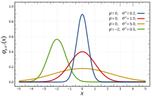
- Normal distribution, Нормальное распределение, распределением Гаусса, bell curve (continuous)(whole real line)
- Notation N(μ,σ^2)
density function (функцией Гаусса):
- PDF f(x) = 1/(σ√(2π))*e^-(x-μ)^2/2σ^2
- CDF F(x) = ….
- μ - mean or expectation of the distribution (and also its median and mode)
- σ - standard deviation
- σ^2 - variance
- Стандартным нормальным распределением называется нормальное распределение с математическим ожиданием μ = 0 и стандартным отклонением σ = 1.
- PDF см 12.9.2 имеет форму колокола x = -∞ to +∞ y = [0;1]
- CDF форму S
- Skewness = 0
Значение:
- Если некая величина образуется в результате сложения многих случайных слабо взаимозависимых величин, каждая из которых вносит малый вклад относительно общей суммы, то центрированное и нормированное распределение такой величины при увеличении числа наблюдений стремится к нормальному распределению.
- to represent real-valued random variables whose distributions are not known
- useful because of the central limit theorem - states that averages of samples of observations of random variables independently drawn from independent distributions converge in distribution to the normal, that is, they become normally distributed when the number of observations is sufficiently large. N(0,1)
- при больших n биноминальная случайная величина приближенно распределена с математическим ожиданием μ=np и стандартным отклонением σ=√(np(1-p))
- Probability density function
- Cumulative distribution function

- Beta distribution
Notation: Beta(α, β)
- defined on the interval [0, 1] or (0, 1)
The beta distribution is a suitable model for the random behavior of percentages and proportions.
http://varianceexplained.org/statistics/beta_distribution_and_baseball/
12.10.3. Сходимость по распределению Convergence of random variables
sequence X1, X2, … of real-valued random variables is said to converge in distribution to a random variable X if:
(n->∞) lim Fn(x) =F(x) where Fn(x) - cumulative distribution functions of random variables Xn and F of X
12.11. Monte Carlo method
чтобы узнать, какое в среднем будет расстояние между двумя случайными точками в круге, методом Монте-Карло, нужно взять много случайных пар точек, для каждой пары найти расстояние, а потом усреднить.
12.12. Law of large numbers Закон больших чисел
the average of the results obtained from a large number of trials should be close to the expected value and tends to become closer to the expected value as more trials are performed.
- LLN only applies to the average.
12.13. Центральная предельная теорема Central limit theorem
It states that, under some conditions, the average of many samples (observations) of a random variable with finite mean and variance is itself a random variable—whose distribution converges to a normal distribution as the number of samples increases.
in many situations, for identically distributed independent samples, the standardized sample mean tends towards the standard normal distribution even if the original variables themselves are not normally distributed.
Неформально говоря, классическая центральная предельная теорема утверждает, что сумма n независимых одинаково распределённых случайных величин имеет распределение, близкое к N(n*μ,n*σ^2)
сумма достаточно большого количества слабо зависимых случайных величин, имеющих примерно одинаковые масштабы (ни одно из слагаемых не доминирует, не вносит в сумму определяющего вклада), имеет распределение, близкое к нормальному.
12.14. Це́пь Ма́ркова Markov chain
последовательность случайных событий с конечным или счётным числом исходов, где вероятность наступления каждого события зависит только от состояния, достигнутого в предыдущем событии
12.15. python PDF, CDF, variance, std
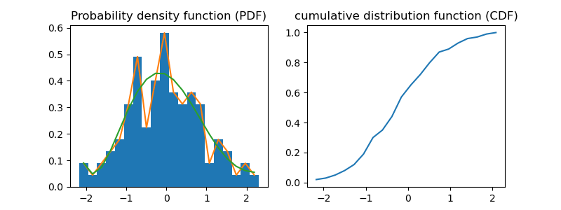
import pandas as pd
import numpy as np
import matplotlib.pyplot as plt
from scipy.interpolate import UnivariateSpline
from math import sqrt
from statistics import variance, stdev

arr = np.random.normal(size=100) # continuous probability mass function
print(pd.Series(arr).describe())

fig = plt.figure(figsize=(8,3))

print(" --------- Probability density function (PDF) or density---------")
print(" - the area under the entire curve is equal to 1")

sp1 = fig.add_subplot(1, 2, 1)   #1 row 2 columns - left
# histogram
sp1.hist(arr, density=True, bins=20)
# line
hist, bin_edges = np.histogram(arr, bins=20, density=True)
x = bin_edges
x = x[:-1] + (x[1] - x[0])/2   # convert bin edges to centers
f = UnivariateSpline(x, hist, k=5)
sp1.plot(x, hist) # line
sp1.plot(x, f(x)) # Spline
sp1.set_title("Probability density function (PDF)")

print(" -------- cumulative distribution function (CDF) ---------")
print(" (x->-∞)lim F(x) = 0 , (x->+∞)lim F(x) = 1")
sp2 = fig.add_subplot(1, 2, 2)   #1 row 2 columns - right

hist, bin_edges = np.histogram(arr, bins=20, density=False)
cumsum = np.cumsum(hist)
cdf = cumsum/cumsum[-1]
sp2.plot(bin_edges[:-1], cdf)
sp2.set_title("cumulative distribution function (CDF)")

# ------ variance -----

print("variance:\t", variance(arr))
# ------ std --------
print("std:\t\t", stdev(arr))

print("sqrt of variance:", sqrt(variance(arr)))
count    100.000000
mean       0.015371
std        1.036308
min       -3.213961
25%       -0.684610
50%       -0.001296
75%        0.618288
max        2.394898
dtype: float64
 --------- Probability density function (PDF) or density---------
 - the area under the entire curve is equal to 1
 -------- cumulative distribution function (CDF) ---------
 (x->-∞)lim F(x) = 0 , (x->+∞)lim F(x) = 1
variance:	 1.073933925916817
std:		 1.0363078335691653
sqrt of variance: 1.0363078335691653
plt.savefig('./autoimgs/pdfcdf.png')
13. Математическая статистика
- родственная теории вероятности
- наблюдая значения случайной величины X, исследователь стремится сделать определенное заключение о неизвестных параметрах вероятностной модели
13.1. terms
- point estimator
- is a function of the random sample that is used to estimate an unknown quantity.
- Q = h(X1, X2, X3) , ex. Q = (X1+X2+X3)/n
13.2. topics wiki
- Descriptive statistics
- Data collection
- Statistical inference
- Frequentist inference
- Bayesian inference
- Statistical theory - probability distribution, bootstrap, loss function
- Correlation
- Regression analysis
- Categorical / Multivariate / Time-series / Survival analysis
13.3. types of statistic:
13.3.1. Statistical inference or inductive statistics
Статистический вывод, индуктивная статистика.
steps:
- select model
- deducing propositions from the model
forms of statistical proposition:
- a point estimate, i.e. a particular value that best approximates some parameter of interest; (Mathematical optimization is a way to solve it)
- interval estimation -
- confidence interval - would contain the true parameter value with the probability at the stated confidence level;
- credible interval, i.e. a set of values containing, for example, 95% of posterior belief;
- distribution estimator - confidence distributions, randomized estimators, and Bayesian posteriors.
- rejection of a hypothesis
- clustering or classification of data points into groups.
- statistical model
statistical model is a set of assumptions concerning the generation of the observed data and similar data. Descriptive statistics are typically used as a preliminary step.
A statistical model is a collection of probability distributions on some sample space.
Degree of models/assumptions
- Fully parametric - all the parameters are in finite-dimensional parameter spaces;
- non-parametric - all the parameters are in infinite-dimensional parameter spaces;
- distribution-free methods
- nonparametric statistics - histogram, etc.
- semi-parametric - finite-dimensional parameters + infinite-dimensional nuisance parameters (parameter which is unspecified)
- semi-nonparametric - finite-dimensional and infinite-dimensional unknown parameters of interest
- paradigs
Bandyopadhyay & Forster describe four paradigms:
- The classical (or frequentist) paradigm
- p-value
- Confidence interval
- Null hypothesis significance testing
- the Bayesian paradigm
- Credible interval for interval estimation
- Bayes factors for model comparison
- the likelihoodist paradigm
- the Akaikean-Information Criterion-based paradigm.
- The classical (or frequentist) paradigm
13.3.2. Descriptive statistics
- does not rest on the assumption that the data come from a larger population.
- aim to summarize a sample.
- not developed on the basis of probability theory, and are frequently nonparametric statistics
measures of
- central tendency - mean, median and mode
- variability or dispersion - standard deviation (or variance), the minimum and maximum values of the variables, kurtosis and skewness
13.4. Statistical inference
is a collection of methods that deal with drawing conclusions from data that are prone to random variation.
ex: Let X be a normal random variable with mean μ = 100 and variance σ^2 = 15. Find the probability that X>110.
we should conclude whether has a normal distribution or not. Now, suppose that we can use the central limit theorem to argue that is normally distributed.
Approaches to estimate some quantity from the data:
- Frequentist (classical) Inference
- unknown quantity is assumed to be a fixed quantity. ? = ? /n
- deals with estimating non-random quantities
- Maximum Likelihood Estimation (MLE),
- Bayesian Inference
- deals with estimating random variables.
- Maximum a Posteriori (MAP),
- Метод максимального правдоподобия maximum likelihood estimation (MLE)
это метод оценивания неизвестного параметра путём максимизации функции правдоподобия - seek a set of parameters that results in the best fit for the joint probability of the data sample (X).
we wish to maximize the probability of observing the data from the joint probability distribution given a specific probability distribution and its parameters
steps:
- defining a parameter called theta that defines both the choice of the probability density function and the parameters of that distribution. It may be a vector of numerical values whose values change smoothly and map to different probability distributions and their parameters.
- P(X | theta) stated using the semicolon (;) notation because theta is not a random variable, but instead an unknown parameter. P(x1, x2, x3, …, xn ; theta) or L(X ; theta)
- to find the set of parameters (theta) that maximize the likelihood function
- The joint probability distribution can be restated as the multiplication of the conditional probability for
observing each example given the distribution parameters.
- product i to n P(xi ; theta)
- Multiplying many small probabilities together can be numerically unstable in practice,. therefore, it is
common to restate this problem as the sum of the log conditional probabilities of observing each example
given the model parameters.
- sum i to n log(P(xi ; theta))
- or minimize -sum i to n log(P(xi ; theta))
13.5. regression analysis
13.5.1. Linear regression
linear approach for modelling the relationship between a scalar response and one or more explanatory variables
y=X*b+ϵ , where
- y - regressand, endogenous variable, response variable, measured variable, criterion variable, or dependent variable
- X - regressors, exogenous variables, explanatory variables, covariates, input variables, predictor variables, or independent variables
- b - parameter vector and ϵ - vector, error term, disturbance term, or noise
13.5.2. General linear models or multivariate linear models (Основная линейная модель)
- y is a vector
- b replaced with B - matrix
13.5.3. Generalized linear model
13.6. Statistical dispersion
zero if all the data are the same and increases as the data become more diverse:
- Standard deviation
- Interquartile range (IQR)
- Range
- Mean absolute difference (also known as Gini mean absolute difference)
- Median absolute deviation (MAD)
- Average absolute deviation (or simply called average deviation)
- Distance standard deviation
13.7. A/B тестированию, Bucket tests, Split-run testing, Раздельное тестирование
13.7.1. terms
- Conversion Rate - dividing the number of desired completed actions by the number of visitors
- multivariate testing - A/B and
13.7.2. definition
представляет собой проверку значимости различия двух реализаций одной и той же случайной переменной
A/B testing is a method of comparing two versions of a webpage or app against each other to determine which one performs better against a specific objective. (more cases = multivariate)
13.7.3. steps
rus
- набор наблюдений, в которых случайная переменная принимает, например, 100 различных значений, случайным образом разделяют на два равных (по 50 наблюдений) подмножества: контрольное A и модифицированное B.
- формулируют гипотезу о значимости их различия относительно дисперсии, среднего или другой структурной характеристики
web
- decide what we would like to test and what our objective is
- we create one or more variations of our original web element (a.k.a. the control group, or the baseline)
- split the website traffic randomly between two variations. Calc:
- необходимый объем выборки
- минимальной разнице в показателях, которую мы хотим выявить, и необходимой статистической мощности
- collect data regarding our web page performance (metrics)
- After some time, we look at the data, pick the variation that performed best, and cancel the one that performed poorly. (calc p-value, также известной как “уровень достоверности)
13.7.4. hypothesis testing
The process of gaining validity is called hypothesis testing, and the validity we seek is called statistical significance.
Неверно, что p-value — это вероятность того, что вариация B лучше, чем вариация A.
“нулевой гипотезе” — которая гласит, что новая вариация ничем не лучше существующей
- Если p-value ниже определенного порога (который часто принимают за 0,05), мы можем утверждать, что данные позволяют опровергнуть нулевую гипотезу и, таким образом, объявить вариацию B победителем
13.7.5. Частотный и байесовский подходы - сравнение
| Hypothesis Testing | Bayesian A/B Testing | |
| Знания о показателях при старт | Нужны | Не нужны |
| Интуитивность | Невысокая p-value - сложная | напрямую вычисляем вероятность, что А лучше B |
| Объем выборки | Определен заранее | Не нужно вычислять заранее |
| подсмотреть в процессе | Нельзя | Можно |
| скорость принятия решения | ниже, больше огран.-щих доп-ий о распр.-ях | выше, меньше допущений |
| Неуверенность выражается | доверительный интервал | область наибольшей апост. плотности (HPDR) |
| Объявление победителя | достигнут объем выборки и p-value < порога | P2BB > порог или когда |
13.7.6. links
- https://www.dynamicyield.com/lesson/introduction-to-ab-testing/
- Hypothesis Testing https://www.dynamicyield.com/lesson/frequentists-approach-to-ab-testing/
- bayesian approach https://www.dynamicyield.com/lesson/bayesian-approach-to-ab-testing/
- bayesian calc https://marketing.dynamicyield.com/bayesian-calculator/
- How Not To Run an A/B Test https://www.evanmiller.org/how-not-to-run-an-ab-test.html
- https://en.wikipedia.org/wiki/Power_of_a_test
- https://vc.ru/u/1174886-koptelnya/411293-chastotnyy-i-bayesovskiy-podhody-k-a-b-testirovaniyu-podrobnoe-sravnenie-urok-7
- article https://wiki.loginom.ru/articles/ab-testing.html
13.8. sample and population
- statistical population - set of items for experiment.
- sample - subset of population
- sampling fraction = len(sample)/len(population)
- sample points - elements of sample
13.9. точечное оценивание (point estimation)
involves the use of sample date to calculate a signle values - best guess of unknown population paremeter
13.10. Estimator [ˈestɪmeɪtə] оценка
Rule for calculating an estimate of a given quantity based on observed data
- estimand - θ - fixed parameter of model being estimated
- estimator q - is a function that maps the sample space to a set of sample estimates
- Error - For a given sample - e(x) = q(x)-θ
- MSE of q - E[(q(X)-θ)^2)]
Types:
- point estimator - single value
- interval estimator - two values
- confidence intervals - Frequentist inference
- credible intervals - Bayesian inference
13.10.1. point estimator
- Bias is defined as the difference between the expected value of the estimator and the true value
of the population parameter being estimated
13.11. интервальное оценивание (interval estimation) - Доверительный интервал
Доверительный интервал - покрывает неизвестный параметр с заданной точностью. Чтобы population parameter попадал в интервал в 95 процентах случаев.
более предпочтителен чем точечние оценивание при небольшой выборке
Различают классический (confidence interval CI) и баесовый интервал (credible interval)
Most commonly 95% confidence level used.
Ex: Here is CI interval from XYZ experiments. Means:
- confidence interval
- If we repeat the experiment infinitely times 95% of calculated intervals will capture parameter in CI. Frequientist. boundaries random, parameter fixed.
- credible interval
- There is 95% probability/plausibility/likelihood that the parameter lies in the interval. Bayesian statistics. Boundaris fixed, variable random.
- confidence interval
- If we repeat the experiment infinitely times 95% of calculated intervals will capture parameter in CI. Frequientist.
13.12. Likelihood and Probability
Понятия вероятности и правдоподобия тесно связаны.
- Вероятность - используется для описания результата функции при наличии фиксированного значения параметра.
- Правдоподобие - используется для описания параметра функции при наличии результата функции.
- «Какова вероятность выпадения 12 очков в каждом из ста бросков двух костей?»
- «Насколько правдоподобно, что кости не шулерские, если из ста бросков в каждом выпало 12 очков?»
Функция правдоподобия Likelihood function
- P(x) = P(x)
- L(q) = L(x=X|q) - показывает, насколько правдоподобно выбранное значение параметра q при известном событии X.
13.13. Statistical hypothesis testing
method of statistical inference used to decide whether the data at hand sufficiently support a particular hypothesis
- statistical inference - статистический вывод process of using data analysis to infer properties of an underlying distribution of probability
- data at hand - имеющиеся данные
- provisional conclusions - предварительные выводы
- statistical independence - probability independence of events
- the null hypothesis (denoted H0) - ('no effect' or 'no difference'). Tested in a test of statistical significance.
- alternative hypothesis (H1 and Ha)
- Test statistic T (Статистический критерий) - математическое правило, в соответствии с которым принимается
или отвергается та или иная статистическая гипотеза с заданным уровнем значимости.
- t-statistic - used in Student's t-test -
- F-test -
Statistical significance(denoted by α or - when it is very unlikely to have occurred given the null hypothesis (simply by chance alone). The significance level α is the threshold for p below which the null hypothesis is rejected even though by assumption it were true, and something else is going on.
- is the probability of the study rejecting the null hypothesis, given that the null hypothesis is true.
- The significance level for a study is chosen before data collection, and is typically set to 5%
- p-value - the probability of obtaining a result at least as extreme, given that the null hypothesis is true. Как я понял, вычеленная вероятность, которая подтвердила null гипотезу оказавшись меньше The significance level.
- One- and two-tailed tests - способ расчета p-value как хвосты нормального распределения - места где значения маловероятны.
p-value vs α:
- p-value is the probability of obtaining a result at least as extreme, given that the null hypothesis is true.
- a - is the probability of the study rejecting the null hypothesis, given that the null hypothesis is true
- The result is statistically significant, by the standards of the study, when p ≤ α.
Fisher's null hypothesis testing
- Do not use a conventional 5% level
- do not talk about accepting or rejecting hypotheses.
- If the result is "not significant", draw no conclusions and make no decisions, but suspend judgement until further data is available
13.13.1. steps:
- state the relevant null and alternative hypotheses
- statistical independence and Statistical assumptions
- Distributional assumptions
- Structural assumptions - relationships between variables
- Cross-variation assumptions -
- Design-based assumptions - the way observations have been gathered
- Decide which test is appropriate, and state the relevant test statistic T
13.13.2. Chi-squared distribution
распределение суммы квадратов k независимых стандартных нормальных случайных величин.
- x = z1^2 + z2^2 + … + zk^2 - случайная величина
- x есть Chi-squared distribution, если z1-k - совместно независимые стандартные нормальные случайные величины N(0,1)
- k степеней свободы
13.13.3. examples
to determine whether a coin flip is fair (equal chance of landing heads or tails) or unfairly biased (one outcome being more likely than the other).
- https://en.wikipedia.org/wiki/P-value
- heads 14 times out of 20 total flips
- null hypothesis is that the coin is fair - coin tosses are independent of one another
- H0: The coin is fair, Pr(heads) = 0.5
- p-value of this result is the chance of a fair coin landing on heads at least 14 times out of 20 flips. This
probability is the p-value, considering only extreme results that favor heads.
- p-value = Pr(14 heads) + Pr(15 heads) + … + Pr(20 heads) ~= 0.058 - one-tailed test
- p-value = 0.115 for two-tailed test
- Test statistic: Number of heads
- Alpha level (designated threshold of significance): 0.05
calculated p-value exceeds .05, meaning that the data falls within the range of what would happen 95% of the time were the coin in fact fair. Hence, the null hypothesis is not rejected at the .05 level.
так как мы задали p-value -
However, had one more head been obtained, the resulting p-value (two-tailed) would have been 0.0414 (4.14%), in which case the null hypothesis would be rejected at the .05 level.
13.13.4. Behrens–Fisher problem
- i.i.d = Independent and identically distributed random variables P(A and B) = P(A)P(B) - independent
- X, Y - iid samples, same location–scale family of distributions
13.14. TODO Power Analysis
- To find the number of trials needed to get an effect of a certain size. This is probably the most common use for power analysis–it tells you how many trials you need to do to avoid incorrectly rejecting the null hypothesis.
- To find the power, given an effect size and the number of trials available. This is often useful when you have a limited budget, for say, 100 trials, and you want to know if that number of trials is enough to detect an effect.
- To validate your research. Conducting power analysis is simply put–good science.
13.15. Resampling
creation of new samples based on one observed sample
13.16. R-squared, Adjusted R-squared and Pseudo-R-squared (coefficient of determination)
the proportion of variance in the response variable y that your regression model is able to “explain” via the introduction of regression variables.
- measure in Regression Analysis
- confused with the coefficient of correlation r²
- R² lets you quantify just how much better the Linear model fits the data as compared to the Mean Model.
Total Sum of Square (TSS). ∑(yi-ymean)^2, where ∑ is for i of N.
- quantity that is proportional to the variance in y
- It is the variance that the Mean Model wasn’t able to explain.
- Because TSS/N is the actual variance in y, the TSS is proportional to the total variance in your data.
Mean Model (Null Model) : y_ped = y_mean
13.17. Confounding
Exposure(воздействие) -> Mediator -> Outcome ( Exposure -> Outcome )
- where -> is cause
Exposure <- Confounder -> Outcome ( Exposure -!- Outcome )
There is no confronder if P(y|do(x)) = P(y|x), where P(y|x) is controlled experiment, with x randomized, do(x) - when x is under the hypothetical intervention.
can be obtained by "adjusting" for all confounding factors, namely, conditioning on their various values and averaging the result.
- P(y|do(x)) = ∑P(y|x,z)P(z), where ∑ at z
14. Calculus Математический анализ (Functional analysis)
14.1. Differential calculus
concerning instantaneous rates of change and slopes of curves - мгновенных скоростей и угловой коэффициент
14.1.1. Gradient or gradient vector field
is a multi-variable generalization of the derivative. While a derivative can be defined on functions of a single variable, for functions of several variables.
Represents the slope of the tangent of the graph of the function. Угловой коэффициент прямой - коэффициент k of f(y)=kx+b численно равен тангенсу угла
nabla ∇f or grad f(x,y,z) = ∂f/∂x(i) +∂f/∂y(j) + ∂f/∂z(k) where i,j,k оси OR вектор (∂f/∂x, ∂f/∂y, ∂f/∂z) - частные производные
f(x,y,z) - называют скалярным полем scalar field
14.2. Vector calculus
- Scalar fields - function that associating a single number to every point in a space
- Vector fields - function that associating a vector to each point in a space
14.3. integral calculus
14.4. Fourier transform (discrete Fourier transform - DFT)
Применяются в сжатии звука в MP3, сжатии изображений в JPEG и др.
Сопоставляющая одной функции вещественной переменной другую функцию вещественной переменной.
14.4.1. Convolution
Mathematical operation on two functions (f and g) that produces a third function expressing how the shape of one is modified by the other
14.4.2. Dirac delta function
function equal to zero everywhere except for zero and whose integral over the entire real line is equal to one