Table of Contents
- 1. Anisotropy image
- 2. Computer vision
- 3. OpenCV
- 3.1. basic
- 3.2. Basic Operations
- 3.3. imread
- 3.4. resize() and interpolation
- 3.5. help libs
- 3.6. install
- 3.7. load save
- 3.8. display
- 3.9. Histogram
- 3.10. Normalize
- 3.11. Contours
- 3.12. Blur
- 3.13. Eroding and Dilating
- 3.14. Features
- 3.15. TODO Filtering
- 3.16. Sobel Derivatives
- 3.17. Colors
- 3.18. template matching
- 3.19. Hough Line Transform
- 3.20. Contrast and brightness
- 3.21. Image Recognition and Object Detection
- 3.22. Generalized Hough Transform - object detection
- 3.23. Cascade of Classifiers - object detection
- 3.24. DNN - object detection
- 3.25. image alignment or Homography
- 3.26. Morphological Transformations
- 3.27. Deep Neural Network module (dnn)
- 3.28. USECASES
- 3.28.1. resize with black are keep ratio
- 3.28.2. subimage
- 3.28.3. scale to target height
- 3.28.4. colours
- 3.28.5. most common colour
- 3.28.6. max x min y
- 3.28.7. Images blending-adding
- 3.28.8. filter contours
- 3.28.9. tables
- 3.28.10. rotate with PIL and Hough Lines
- 3.28.11. PIL convert
- 3.28.12. rotate
- 3.28.13. resize, shift-translate, shrinking with warpAffine
- 3.28.14. Lines
- 3.28.15. minAreaRect
- 3.28.16. detect shape of contour
- 3.28.17. detect objects by shape (link)
- 3.28.18. image to batch
- 3.28.19. cut part of image
- 3.29. troubleshooting
- 4. MMCV
- 5. Abby
- 6. Rusnarbank_OPENCV
- 7. passport
- 8. captcha
- 9. optical label
- 10. OCR ICR
- 11. подпись signature (ˈsɪɡnətʃər;) handwritten
- 12. 12 лучших репозиториев GitHub по компьютерному зрению
- 13. VR
- 14. NEXT LEVEL
-- mode: Org; fill-column: 110; coding: utf-8; --
bible https://docs.opencv.org/
https://stackoverflow.com/questions/40192541/how-to-detect-the-bounds-of-a-passport-page-with-opencv
TODO Уменьшение яркости и повышение контрастности для устранения фоновых артефактов. https://ru.stackoverflow.com/questions/377281/%D0%A0%D0%B0%D1%81%D0%BF%D0%BE%D0%B7%D0%BD%D0%B0%D0%B2%D0%B0%D0%BD%D0%B8%D0%B5-%D1%82%D0%B5%D0%BA%D1%81%D1%82%D0%B0-%D0%BD%D0%B0-%D0%BE%D1%82%D1%81%D0%BA%D0%B0%D0%BD%D0%B8%D1%80%D0%BE%D0%B2%D0%B0%D0%BD%D0%BD%D0%BE%D0%BC-%D0%BF%D0%B0%D1%81%D0%BF%D0%BE%D1%80%D1%82%D0%B5
1. Anisotropy image
Anisotropy (ænɪˈsɒtrəpi) - different properties in different directions
- structure tensor - matrix derived from the gradient of a function.
- tensor - algebraic object that describes a multilinear relationship between sets of algebraic objects related to a vector space
- Multilinear map - function of several variables that is linear separately in each variable. f:V1xV2.. -> W
- for each i, if all of the variables but Ui are held constant, then f(U1,U2..) is linear function of Ui.
- Multilinear map - function of several variables that is linear separately in each variable. f:V1xV2.. -> W
- Gradient - of a scalar-valued differentiable function f of several variables is the vector field (or
vector-valued function) ∇f (nabla) whose value at a point p is the vector whose components are the *partial
derivatives of f at p.
- f:Rn -> R, its gradient ∇f:Rn -> Rn.
- at point p: ∇f(p) = [ df(p)/dx1, … df(p)/dxn ]
- Partial derivative - of a function of several variables is its derivative with respect to one of those variables, with the others held constant. df/dx
- tensor - algebraic object that describes a multilinear relationship between sets of algebraic objects related to a vector space
Scale space - for handling image structures at different scales - Gaussian derivative operators, can be used as a basis for expressing a large class of visual operations
2. Computer vision
Computer vision - high-level understanding from digital images or videos
- Digital image processing - to process digital images through an algorithm.
2.1. Steps of image processing:
- image smoothed by a Gaussian kernel in a scale-space representation
- threshold or canny edge detection filters
- features extracting
- path around the feature - feature descriptor or feature vector. - N-jets and local histograms
- specific algoriths
2.2. CV LIBRARIES
- OpenCV C C++ Python
- Caffe C++ Python Matlab - быстрая на С++
- Torch7
- clarifai
- Google Vision API
2.3. image CV_8U, CV_32F
usually numpy array of image data:
- CV_8U: 1-byte unsigned integer (unsigned char).
- CV_32S: 4-byte signed integer (int).
- CV_32F: 4-byte floating point (float).
2.3.1. convert
print(img.dtype) >>> float32 img.astype(np.uint8)
2.4. Color models
2.4.1. CIE XYZ color space
Исторически сложилось, XYZ - эталонная цветовая модель организациии CIE (commission internationale d'eclairage)— Международная комиссия по освещению) в 1931 году.
Иногда используют xyY представление XYZ. Если Y = const, можно изобразить все возможные монохроматические цвета спектра, то они образуют собой незамкнутый контур, так называемый спектральный локус.
- Y - светлота
- x - X/(X+Y+Z)
- y - Y/(X+Y+Z)
- RGB - 24-bit - 8 bits, for red, green, and blue
2.4.2. RGB
red, green, blue
- tupically 24-bit RGB or 32-bit RGBA colors
- 8+8+8 (sRGB - 8 bits per channel)
RGBA32 or ARGB - with alpha channel
- alpha channel - transparency
2.4.3. HSV
Сделан чтобыпроще понять человеку как сделать цвет и отдельно яркость
- hue - тон - угол [0,360] - binary [0,255]
- 0 - red
- 60 yellow
- 120 green
- 180 blue
- 240 dark blue
- 300 purple
- saturation - насыщенность - [0,1] - binary [0,255]
- value(brightness) - [0,1] - binary [0,255]
center - neutral - black at bottom, white at top
hue:
- NewValue = (((OldValue - OldMin) * NewRange) / OldRange) + NewMin
- (((120 - 0) * 255)/360) + 0 = 85
2.5. OpenCV techs
2.5.1. Histogram Equalization
http://datahacker.rs/opencv-histogram-equalization/ https://ru.qaz.wiki/wiki/Histogram_equalization
- inrease contrast
- Этот метод полезен для изображений с ярким или темным фоном и передним планом.
- хорошо работает с высокой глубиной цвета
- может увеличить контраст фонового шума и уменьшить полезный сигнал
2.5.2. TODO image segmentation
2.5.3. TODO extract features
2.5.4. Discrete Fourier Transform, ряд Фурье
http://datahacker.rs/opencv-discrete-fourier-transform-part1/ http://datahacker.rs/opencv-discrete-fourier-transform-part2/
- time-domain analysis shows how a signal changes over time
- frequency-domain analysis shows how the signal’s energy is distributed over a range of frequencies
2.6. Основные преобразования 2 di
Непрерывное отображение
- гомеоморфизмом - имеет непрерывное обратное
Homography - Проективное преобразование
- прямые в прямые
- Allow to manipulate n‐dim vectors in a n+1 dim space
- 2 degrees of freedom
- homogeneous image coordinates = (x,y,1) - column
- Converting from homogeneous image coordinates (x,y,1) = (x/w,y/w)
- Transformation = (x,y,1) * 3x3 matrix -> (x/w,y/w)
affine transformation
- preserves:
- points
- straight lines
- planes
- parallelism
- include: translation, scaling, homothety, similarity transformation, reflection, rotation, shear mapping, and compositions
- affine transformation matrix - последняя строка [001]
- projective transformation matrix
2.6.1. linear transformation (Linear map) - линейный оператор
rotation point (x/y) 2 dim, θ - от x+ оси (one degree of freedom):
- [ cos -sin ] x = x*cosθ - y*sinθ
- [ sin cos ] y = x*sinθ + y*cosθ
Reflection
caling by 2
- [2 0]
- [0 2]
horizontal shear mapping - Горизонтальный сдвиг
- [1 m]
- [0 1]
squeeze mapping
- [k 0]
- [0 1/k]
projection onto the y axis:
- [0 0]
- [0 1]
2.7. feature detection
Types of image features:
- Edges
- Canny edge detector
- Corners / interest points
- point-like features, early algorithms first performed edge detection, and then analysed the edges to find rapid changes in direction (corners)
- Blobs / regions of interest points
- complementary description of image structures in terms of regions. Just like edge
- Ridges
- represents an axis of symmetry has an attribute of width associated with each ridge point - algorithmically harder to extract
2.8. Optical Character Recognition
- handwritten or printed text into machine-encoded text
- распознавание латинских символов в печатном тексте в настоящее время возможно, только если доступны чёткие изображения, такие, как сканированные печатные документы. Точность при такой постановке задачи превышает 99 %
- рукописного «печатного» и стандартного рукописного текста, а также печатных текстов других форматов (особенно с очень большим числом символов) в настоящее время являются предметом активных исследований
2.9. datasets
Berkeley Segmentation Data Set and Benchmarks 500 (BSDS500) https://www2.eecs.berkeley.edu/Research/Projects/CS/vision/grouping/resources.html
2.10. USECASES
2.10.1. rotate
array([1, 2], [3, 4])
np.rot90(m) array([2, 4], [1, 3]])
2.10.2. boxes with check mark (check box) or with text
2.11. links
3. OpenCV
- hpp usr/include/opencv4/opencv2
- tpoint https://www.tutorialspoint.com/opencv/index.htm
- doc https://www.docs.opencv.org/master/
- doc https://docs.opencv.org/4.8.0/d9/df8/tutorial_root.html
- Doc numpy https://docs.scipy.org/doc/numpy/reference/arrays.ndarray.html
- https://ru.wikipedia.org/wiki/OpenCV
- https://gitlab.rusnarbank.ru/m.smirnov/Rusnarbank_OPENCV
- https://www.pyimagesearch.com/2018/08/20/opencv-text-detection-east-text-detector/
- шпаргалка https://tproger.ru/translations/opencv-python-guide
- imutils - Adrian Rosebrock https://github.com/jrosebr1/imutils
3.1. basic
- Region of interest (ROI)
- color-space conversion
- RGB - 24-bit - 8 bits, for red, green, and blue
- HSV - hue, saturation, value. OpenCV uses HSV ranges between (0-180, 0-255, 0-255).
- binary images - 0,1 or 0,255
- gray image - single channels 8-bit image
- Morphological Transformations - performed on binary images
- Gradient filters or High-pass filters
- Sobel
- Scharr
- Laplacian
- Thresholding filter - grayscale image -> If pixel value is greater than a threshold value, it is assigned one value (may be white), else it is assigned another value (may be black). -> grayscale or binary image AND retVal -
- bimodal image is an image whose histogram has two peaks
- Canny edge detection - argument: min and max values - Noise Reduction, Intensity Gradient
- Image Pyramids - Higher level (Low resolution)
- Gaussian Pyramid - higher level is formed by the contribution from 5 pixels with gaussian weights - rediced to one-fourth of original area MxN -> M/2,N/2 - cv.pyrDown() and cv.pyrUp()
- Laplacian Pyramids - images are like edge images only
- Contours - curve joining all the continuous points - for shape analysis and object detection and recognition.
де-факто, стандартом в области компьютерного зрения
- is written in C++ and its primary interface is in C++
- Python, Java and MATLAB/OCTAVE
- CUDA-based GPU and OpenCL-based GPU interfaces
- Windows, Linux, macOS, FreeBSD, NetBSD, OpenBSD
- Android, iOS, Maemo, BlackBerry 10
EAST EAST: An Efficient and Accurate Scene Text Detector.
- OpenCV 3.4.2 and OpenCV 4
- arbitrary orientations
- 720p images
3 ways to document recognation
- AKAZE + rectangles template
- search rectangle by text with gradients or threshold
- search text in areas with tesseract detected text
3.1.1. DPI
dpi is just a number in the JPEG/TIFF/PNG header
DPI - scale factor to convert inches coordinates into pixel coordinates and back
OpenCV doesn't know about DPI
3.2. Basic Operations
- BGR image - 3d
- grayscale image - 1d
img.shape = (height, width, channels) = (rows, cols, channels)
cv.resize(img, (width, height))
import numpy as np
import cv2 as cv

img = cv.imread('messi5.jpg')  # numpy.ndarray - type
px = img[100,100]   #[157 166 200] - Blue, Green, Red
img.item(10,10,2)   # red value of pixel
img.itemset((10,10,2),100)   # set red value of pixel
print( img.shape )  # (342, 548, 3)
print( img.size )   # 562248
print( img.dtype )  # uint8 or cv.CV_8U

b,g,r = cv.split(img) # Blue, Green, Red
b = img[:,:,0] # faster
img = cv.merge((b,g,r))

cv2.imshow('image',img) # show image in window
cv2.waitKey(0)          # wait for any key indefinitely
cv2.destroyAllWindows() # close window

from matplotlib import pyplot as plt
plt.imshow(img, cmap = 'gray', interpolation = 'bicubic')
plt.xticks([]), plt.yticks([])  # to hide tick values on X and Y axis
plt.show()

#color-space conversion
# HSV or HSB - тон (1-360), насыщенность(0-100)(0-серый), яркость(0-100)
hsv = cv.cvtColor(input_image,  cv.COLOR_BGR2HSV) # convert, cv.COLOR_BGR2GRAY
lower_blue = np.array([110,50,50])
upper_blue = np.array([130,255,255])
mask = cv.inRange(hsv, lower_blue, upper_blue) # Threshold the HSV image to get only blue colors
res = cv.bitwise_and(frame,frame, mask= mask) # original minus mask

bgr_green = np.uint8([[[0,255,0 ]]]) # BGR: Green
hsv_green = cv.cvtColor(green,cv.COLOR_BGR2HSV) # [[[ 60 255 255]]]

# THRESH_BINARY = maxval if pix > thresh else 0
ret,thresh1 = cv.threshold(src=img, thresh=127, maxval=255, type=cv.THRESH_BINARY)
3.3. imread
- BGR order and its cv2.imshow() and cv2.imwrite() also expect images in BGR order.
- Other libraries, such as PIL/Pillow, scikit-image, matplotlib, pyvips store images in conventional RGB order in memory.
img = cv.imread(p, cv.IMREAD_COLOR)
[[ [250 250 250] … ] … ]
convert to RGB:
- RGBimage = cv2.cvtColor(BGRimage, cv2.COLOR_BGR2RGB)
3.4. resize() and interpolation
https://chadrick-kwag.net/cv2-resize-interpolation-methods/
- INTER_NEAREST – a nearest-neighbor interpolation
- INTER_LINEAR – a bilinear interpolation (used by default)
- INTER_AREA – resampling using pixel area relation. It may be a preferred method for image decimation, as it gives moire’-free results. But when the image is zoomed, it is similar to the INTER_NEAREST method.
- INTER_CUBIC – a bicubic interpolation over 4×4 pixel neighborhood
- INTER_LANCZOS4 – a Lanczos interpolation over 8×8 pixel neighborhood
3.5. help libs
3.6. install
sudo apt-get install libopencv-dev python-opencv
3.7. load save
img = cv.imread('messi5.jpg', flag) # as a multi-dimensional NumPy array BGR order
flags: https://docs.opencv.org/4.1.0/d6/d87/imgcodecs_8hpp.html
- cv.IMREAD_COLOR : transform to BGR colours. Any transparency of image will be neglected. It is the default flag.
- cv.IMREAD_GRAYSCALE = 0 : Loads image in grayscale mode
- cv.IMREAD_UNCHANGED : Loads image as such including alpha channel
cv2.imwrite('messigray.png', crop_box)
3.8. display
self.contours = np.array(list(filter(lambda x: x is not None, self.contours)))
self.img[:] = 255
cv2.drawContours(self.img, self.contours, -1, (0, 255, 0), 10)
cv2.imshow('image', self.img)  # show image in window
cv2.waitKey(0)  # wait for any key indefinitely
cv2.destroyAllWindows()  # close window

from matplotlib import pyplot as plt

img = cv2.cvtColor(image, cv2.COLOR_BGR2RGB)
plt.imshow(image)
plt.axis("off")
plt.show()

# несколько
plt.subplot(121) # два изображения по горизонтали, 211 - два изображения по вертикали
plt.imshow(img)
plt.subplot(122)
plt.plot(hist) # граффик
plt.xlim([0,256]) # обл допус знач ось X
plt.show()


self.cluster_coords = [[  9.  622. ],[  9.  563.5]]
pts = np.array([self.cluster_coords], np.int32)
cv2.drawContours(self.img, pts, -1, (0, 255, 0), 3)
img = cv2.resize(self.img, (700, 800)) #resize if too large
cv2.imshow('image', img)  # show image in window
cv2.waitKey(0)  # wait for any key indefinitely
cv2.destroyAllWindows()  # close window


# contour to rectangle
x, y, w, h = cv2.boundingRect(contour)
cv2.rectangle(img, (x, y), (x+w, y+h), (0, 255, 0), 2)
3.9. Histogram
- pixel value - 0-255
- histogram - for grayscale image mostly - intensity distribution of an image - x - 0 to 255, у - number of pixels
- BIN - number of pixel values. группировка values - [256] - количество values в одном ящике
- RANGE : It is the range of intensity values you want to measure. Normally, it is [0,256], ie all intensity values.
cv.calcHist(images, channels, mask, histSize, ranges[, hist[, accumulate]])
- mask : mask image. To find histogram of full image, it is given as "None".
- histSize : this represents our BIN count. Need to be given in square brackets. For full scale, we pass [256].
- ranges : this is our RANGE. Normally, it is [0,256].
BGR:
cv.calcHist(images=[img], chnnels=[i], mask=None, histSize=[256], ranges=[0, 256])
HSV:
hist = cv.calcHist(images=[hue], chnnels=[0], mask=None, histSize=[2-180], ranges=[0, 180])
- histSize - bins
from matplotlib import pyplot as plt
import cv2 as cv
img = cv.imread('/home/u/sources/tasks-for-job/task_for_zennolab/train.png', 0)
#img = cv.imread('/home/u/download.jpeg', 0)
hist = cv.calcHist([img],[0],None,[256],[0,256])
plt.subplot(121)
plt.imshow(img)
plt.subplot(122)
plt.plot(hist)
plt.xlim([0,256])
plt.show()
3.10. Normalize
cv2.normalize(source_array, destination_array, alpha, beta, normType )
- source_array
- It is the input image you want to normalize.
- destination_array
- The name for the output image after normalization.
- alpha
- norm value to normalize to or the lower range boundary in case of the range normalization.
- beta
- upper range boundary in case of the range normalization; it is not used for the norm normalization.
- normType
- Type for the normalization of the image.
- cv2.NORM_MINMAX
Don't change:
norm = np.zeros((800,800)) #  blank image
norm_image = cv2.normalize(img,norm,alpha=0,beta=255,cv2.NORM_MINMAX) # img -BGR
To convert each pixel to 0-1 range:
img_normalized = cv2.normalize(img, None, 0, 1.0, cv2.NORM_MINMAX)
3.11. Contours
cv.findContrours
contours, hierarchy = cv.findContours(thresh, cv.RETR_TREE, cv.CHAIN_APPROX_SIMPLE) # finding white object from black background
- input - binary image - 0 - BLACK, 255 - WHITE
- cv.RETR_TREE - contour retrieval mode -
- https://docs.opencv.org/4.1.0/d9/d8b/tutorial_py_contours_hierarchy.html
- list of contours
- [8, 0, -1, -1] -0: 8 next in same hoerarchy, 0 previous in same hoerarchy, -1 no child, no parent
- [-1, -1, 3, 1] -1: -1 no next, -1 no previous, 3 is a child, 1 is a parent
- cv.CHAIN_APPROX_SIMPLE - contour approximation method - all the boundary points are stored, or several
- cv.CHAIN_APPROX_SIMPLE - removes all redundant points and compresses the contour, thereby saving memory
- contours - list of all the contours. Each individual contour is a Numpy array of (x,y) coordinates
- example for contours parameter: [[[ 22 124] [ 57 160]]]
contours = [numpy.array([[1,1],[10,50],[50,50]], dtype=numpy.int32) , numpy.array([[99,99],[99,60],[60,99]], dtype=numpy.int32)]
cv.drawContours - around or inside of contour
cv.drawContours(img, [contours[0]], 0, (255), -1)
- 0 - draw first contour of [contours[0]] (-1 - all)
- (255) - colour to draw
- -1 - thinkness - if -1 - draw inside contour
to rectangle:
x,y,w,h = cv.boundingRect(cnt)
3.11.1. working with contours
img = cv.imread('/home/u/sudou2.jpg', 0)
ret, thresh = cv.threshold(img, 127, 255, 0)
contours, hierarchy = cv.findContours(thresh, cv.RETR_EXTERNAL, cv.CHAIN_APPROX_SIMPLE)
cv.drawContours(img, contours, -1, (0,255,0), 3) # -1 - all, 3 - draw 4th contour
# draw 4th contour
cnt = contours[4]
cv.drawContours(img, [cnt], 0, (0,255,0), 3)

cv.imshow('image', img)  # show image in window
cv.waitKey(0)  # wait for any key indefinitely
cv.destroyAllWindows()  # close window

# one format to another
[x, y, w, h] = cv2.boundingRect(contour)
img = img[item[1]:item[1] + item[3], item[0]: item[0] + item[2]]
img = img[y:y + h, x: x + w] # crop rect

center, size, theta = cv2.minAreaRect(coords) # ( center (x,y), (width, height), angle of rotation )
# Convert to int
center, size = tuple(map(int, center)), tuple(map(int, size))

# contour with angle
rect = cv2.minAreaRect(coords)
box = cv2.boxPoints(rect)
box = np.int0(box)
img2 = self.image.copy()
cv2.drawContours(img2, [box], 0, (0, 0, 255), 2)
cv2.imshow('image', img2)  # show image in window
cv2.waitKey(0)  # wait for any key indefinitely
cv2.destroyAllWindows()  # close window

# EXTERNAL contours
(_, cnts, hierarchy) = cv.findContours(image, cv.RETR_EXTERNAL, cv.CHAIN_APPROX_SIMPLE)
3.11.2. get example of contour
# img_onechannel = img[0]
# ret, thresh = cv.threshold(img_onechannel, 29, 255, 0)
# contours, hierarchy = cv.findContours(thresh, cv.RETR_TREE, cv.CHAIN_APPROX_SIMPLE)
3.12. Blur
convolving (each element of the image is added to its local neighbors, weighted by the kernel) the image through a low pass filter kernel.
- Blur (Averaging) - cv.blur
- pixel replecead by the average of all the pixels in the kernel area
- cv.GaussianBlur
3.13. Eroding and Dilating
- Dilation
- make white lines FAT
- Erosion
- make THIN
https://docs.opencv.org/3.4/db/df6/tutorial_erosion_dilatation.html
3.14. Features
Good features: corners, …
- Feature Detection - create
- Feature Description - describe the region around the feature so that it can find it in other images
- Feature matching
3.14.1. algos:
- Harris Corner Detection - |R| is small->flat, R<0 -> edge, R is large -> corner - rotation-invariant, not scale invariant.
- cv.goodFeaturesToTrack() - find corners for - for tracking - rotation-invariant, not scale invariant.
SIFT - scale invariant.
- Each keypoint is a special structure which has many attributes like its (x,y) coordinates, size of the
meaningful neighbourhood, angle which specifies its orientation, response that specifies strength of keypoints etc.
- SURF - speeded-up version of SIFT
- ORB is much faster than SURF and SIFT and ORB descriptor works better than SURF
3.14.2. matches
Brute-Force Matcher one feature from 1 set match with all other features in second set. Closes is returned.
- bf = cv.BFMatcher(cv.NORM_HAMMING, crossCheck=True)
- match alternatives:
- DMatch - result of bf.match(des1,des2)
- BFMatcher.knnMatch() to get k best matches, so we can apply ratio test.
FLANN Matcher - faster, uses Approximate Nearest Neighbors
matcher.match(queryDescriptors,trainDescriptors)
3.14.3. DMatch
kp1, des1 = sift.detectAndCompute(img1,None)
kp1 - (< cv2.KeyPoint 0x7f214cbb2d90>, < cv2.KeyPoint 0x7f214cf18ae0>, …)
des1 - distances matrix
matches = flann.knnMatch(des1,des2,k=2)
matches - (< cv2.DMatch 0x7f214c2362d0>, < cv2.DMatch 0x7f214c236510>)
source and target points:
for m, n in nn_matches:
    matched1.append(kpts1[m.queryIdx])
    matched2.append(self.kpts2[m.trainIdx])

# ordered lists
src_pts = [i.pt for i in matched1]
dst_pts = [i.pt for i in matched2]
3.15. TODO Filtering
3.16. Sobel Derivatives
express pixel intensity changes
3.17. Colors
3.17.1. channels
color = ('b', 'g', 'r')
for i, col in enumerate(color):
b = (np.ones((500, 500)) * characters[0]).astype(np.uint8)
        g = (np.ones((500,500)) * characters[1]).astype(np.uint8)
        r = (np.ones((500, 500)) * characters[2]).astype(np.uint8)
b = img[:,:, 0]
g = img[:,:, 1]
r = img[:,:, 2]

# back to image
b = np.ones((500, 500)).astype(np.uint8)
g = np.ones((500,500)).astype(np.uint8)
r = np.ones((500, 500).astype(np.uint8)

bgr = np.dstack((b, g, r))
3.17.2. histogram
# gray histogram
hist = cv2.calcHist([gray], [0], None, [256], [0, 256])
plt.figure()
plt.title("Grayscale Histogram")
plt.xlabel("Bins")
plt.ylabel("# of Pixels")
plt.plot(hist)
plt.xlim([0, 256])

# Colours flattened histogram
for (chan, color) in zip(chans, colors):
        # create a histogram for the current channel and
        # concatenate the resulting histograms for each
        # channel
        hist = cv2.calcHist([chan], [0], None, [256], [0, 256])
        features.extend(hist)

        # plot the histogram
        plt.plot(hist, color = color)
        plt.xlim([0, 256])
plt.show()


# Select objects by colour
   lower = np.array([120, 57, 110])  # -- Lower range -- RGB
    upper = np.array([180, 136, 170])  # -- Upper range --
    mask = cv.inRange(img, lower, upper)
    res = cv.bitwise_and(img, img, mask=mask)
    cv.imshow("images", np.hstack([img, res]))
    cv.waitKey(0)
3.18. template matching
- it does not work for rotated or scaled versions of the template
- inefficient when calculating the pattern correlation image for medium to large images
Binary-string descriptors: ORB, BRIEF, BRISK, FREAK, AKAZE, etc.
- use FLANN + LSH index or Brute Force + Hamming distance.
Floating-point descriptors: SIFT, SURF, GLOH, etc.
- Hamming distance as opposed to Euclidean distance used for floating-point descriptors.
3.19. Hough Line Transform
image, rho, theta, threshold, lines=None, srn=None, stn=None, min_theta=None, max_theta=None
- image-edges: Output of the edge detector.
- rho: Distance resolution of the accumulator in pixels. = 1
- theta: Angle resolution of the accumulator in radians. = np.pi/180
- threshold: Accumulator threshold parameter. Only those lines are returned that get enough votes
- lines: A vector to store the coordinates of the start and end of the line. Each line is represented by a 2 or 3 element vector
- stn, srn: For the multi-scale Hough transform,
- min_theta: For standard and multi-scale Hough transform, minimum angle to check for lines. Must fall between 0 and max_theta.
- max_theta: For standard and multi-scale Hough transform, maximum angle to check for lines. Must fall between min_theta and CV_PI
threshold: The minimum number of intersecting points to detect a line.
img = cv.imread('/home/u/download.jpeg', 0)
edges = cv.Canny(img,50,150,apertureSize = 3)
#lines = cv.HoughLines(edges,1,np.pi/180,200)
lines = cv.HoughLinesP(edges,1,np.pi/180,100,minLineLength=100,maxLineGap=10)

for line in lines:
    x1,y1,x2,y2 = line[0]
    cv.line(img,(x1,y1),(x2,y2),(0,255,0),2)

plt.imshow(img)
plt.show()


gray = cv.cvtColor(img,cv.COLOR_BGR2GRAY)
edges = cv.Canny(gray,50,150, apertureSize = 3)
print(edges.shape)
lines = cv.HoughLines(edges,1,np.pi/180,120)
print(lines)
for line in lines:
    rho, theta = line[0]
    a = np.cos(theta)
    b = np.sin(theta)
    x0 = a*rho
    y0 = b*rho
    x1 = int(x0 + 1000*(-b))
    y1 = int(y0 + 1000*(a))
    x2 = int(x0 - 1000*(-b))
    y2 = int(y0 - 1000*(a))
    cv.line(img,(x1,y1),(x2,y2),(0,0,255),2)

#plt.imshow(edges)
plt.imshow(img)
plt.show()
3.20. Contrast and brightness
import cv2 as cv


def funcBrightContrast(bright=0):
    bright = cv.getTrackbarPos('bright', 'Life2Coding')
    contrast = cv.getTrackbarPos('contrast', 'Life2Coding')

    effect = apply_brightness_contrast(img, bright, contrast)
    cv.imshow('Effect', effect)


def apply_brightness_contrast(input_img, brightness=255, contrast=127):
    brightness = map(brightness, 0, 510, -255, 255)
    contrast = map(contrast, 0, 254, -127, 127)

    if brightness != 0:
        if brightness > 0:
            shadow = brightness
            highlight = 255
        else:
            shadow = 0
            highlight = 255 + brightness
        alpha_b = (highlight - shadow) / 255
        gamma_b = shadow

        buf = cv.addWeighted(input_img, alpha_b, input_img, 0, gamma_b)
    else:
        buf = input_img.copy()

    if contrast != 0:
        f = float(131 * (contrast + 127)) / (127 * (131 - contrast))
        alpha_c = f
        gamma_c = 127 * (1 - f)

        buf = cv.addWeighted(buf, alpha_c, buf, 0, gamma_c)

    # cv2.putText(buf, 'B:{},C:{}'.format(brightness, contrast), (10, 30), cv2.FONT_HERSHEY_SIMPLEX, 1, (0, 0, 255), 2)
    return buf


def map(x, in_min, in_max, out_min, out_max):
    return int((x - in_min) * (out_max - out_min) / (in_max - in_min) + out_min)


if __name__ == '__main__':
    original = cv.imread("/mnt/hit4/hit4user/PycharmProjects/cnn/samples/passport_and_vod/0/2019080129-2-0.png", 1)
    original = cv.resize(original, (900, 900))

    # my
    # tmp = apply_brightness_contrast(original, brightness=230, contrast=255)
    # cv.imshow('a', tmp)
    # cv.waitKey(0)

    img = original.copy()

    cv.namedWindow('Life2Coding', 1)

    bright = 255
    contrast = 127

    # Brightness value range -255 to 255
    # Contrast value range -127 to 127

    cv.createTrackbar('bright', 'Life2Coding', bright, 2 * 255, funcBrightContrast)
    cv.createTrackbar('contrast', 'Life2Coding', contrast, 2 * 127, funcBrightContrast)
    funcBrightContrast(0)
    cv.imshow('Life2Coding', original)
    cv.waitKey(0)
3.21. Image Recognition and Object Detection
- https://www.learnopencv.com/image-recognition-and-object-detection-part1/
- https://habr.com/ru/post/208090/
- https://www.pyimagesearch.com/2014/11/10/histogram-oriented-gradients-object-detection/
History:
- 2001 face detection Viola and Jones algorithm
- 2005 Histograms of Oriented Gradients (HOG)
- 2012 ImageNet
Methods:
- Preprocessing
- cropped
- resizing
- RGB to gray
- gamma correction
Filtering OR Feature Extraction
- Бинаризация по порогу (threshold)
- Haar-like features introduced by Viola and Jones
- Histograms of Oriented Gradients (HOG)
- Scale-Invariant Feature Transform ( SIFT )
- Speeded Up Robust Feature ( SURF )
- Фурье, ФНЧ, ФВЧ
- вейвлет-анализом называется поиск произвольного паттерна на изображении при помощи свёртки с моделью этого паттерна
- Edge detector (Мат аппарат - контурный анализ)
- Оператор Кэнни
- Оператор Собеля
- Оператор Лапласа
- Оператор Прюитт
- Оператор Робертса
- Особые точки https://en.wikipedia.org/wiki/Feature_detection_(computer_vision)
- Первый класс. Особые точки, являющиеся стабильными на протяжении секунд.
- локальные максимумы изображения
- углы на изображении (лучший из детекторов, пожалуй, детектор Хариса)
- точки в которых достигается максимумы дисперсии
- определённые градиенты
- Второй класс. Особые точки, являющиеся стабильными при смене освещения и небольших движениях объекта.
- некоторые вейвлеты, как база для точек
- точки, найденные методом HOG
- Третий класс. Стабильные точки.
- SURF, SIFT - К сожалению эти методы запатентованы. Хотя, в России патентовать алгоритмы низя, так что для внутреннего рынка пользуйтесь.
- KAZE and A-KAZE - no patent
- Первый класс. Особые точки, являющиеся стабильными на протяжении секунд.
- Mathematical morphology
of the shape and aim to find out its location and orientation in the image
- Trainging Classificator
- Faster R-CNN has two networks: region proposal network (RPN) for generating region proposals and a network using these proposals to detect objects.
HOG Histograms of Oriented Gradients метод гистограмм направленных градиентов
- based on the idea: that local object appearance can be effectively described by the distribution ( histogram ) of edge directions ( oriented gradients )
- 64 x 128 x 3 = 24,576 which is reduced to 3780
Mathematical morphology
- это простейшие операции наращивания и эрозии бинарных изображений
Template matchong and Object detection
- Hough transform: cv.HoughCircles, cv.HoughLines, cv.HoughLinesP
- Generalized Hough Transform - cv::GeneralizedHoughBallard, cv::GeneralizedHoughGuil. - we have knowledge of the shape and aim to find out its location and orientation in the image.
- https://habr.com/ru/post/113626/
- http://wiki.technicalvision.ru/index.php/%D0%9C%D0%BE%D1%80%D1%84%D0%BE%D0%BB%D0%BE%D0%B3%D0%B8%D1%87%D0%B5%D1%81%D0%BA%D0%B8%D0%B5_%D0%BE%D0%BF%D0%B5%D1%80%D0%B0%D1%86%D0%B8%D0%B8_%D0%BD%D0%B0_%D0%B1%D0%B8%D0%BD%D0%B0%D1%80%D0%BD%D1%8B%D1%85_%D0%B8%D0%B7%D0%BE%D0%B1%D1%80%D0%B0%D0%B6%D0%B5%D0%BD%D0%B8%D1%8F%D1%85
3.22. Generalized Hough Transform - object detection
- cv::GeneralizedHoughBallard - find exactly
- cv::GeneralizedHoughGuil - very slow, find same, not exactly
https://docs.opencv.org/4.8.0/da/ddc/tutorial_generalized_hough_ballard_guil.html
3.23. Cascade of Classifiers - object detection
disabled since OpenCV 4.0!!! via DNN provides much better results
Haar features. paper, "Rapid Object Detection using a Boosted Cascade of Simple Features" in 2001
require usage: media-libs/opencv gtk3 opencvapps
3.23.1. train
training window size - the average size of your object
- positive - opencv_createsamples
- "file of list": file instances_count x y width height
- img/img2.jpg 2 100 200 50 50 50 30 25 25
- negative
- "file of list": one image path per line
- different sizes - each image should be equal or larger than the desired "training window size"
/negative img1.jpg img2.jpg neg.txt
/positive img1.jpg img2.jpg pos.dat
positives: The object instances are taken from the given images, by cutting out the supplied bounding boxes from the original images. Then they are resized to target samples size (defined by -w and -h) and stored in output vec-file, defined by the -vec parameter. No distortion is applied, so the only affecting arguments are -w, -h, -show and -num.
- opencv_createsamples -info pos.dat
- -vec <vec_file_name> : Name of the output file containing the positive samples for training.
- -num <number_of_samples> : Number of positive samples to generate.
- -maxidev <max_intensity_deviation> : Maximal intensity deviation of pixels in foreground samples.
- -show : Useful debugging option. If specified, each sample will be shown. Pressing Esc will continue the samples creation process without showing each sample.
- -w <sample_width> : Width (in pixels) of the output samples.
- -h <sample_height> : Height (in pixels) of the output samples.
opencv_createsamples -info pos.dat -vec a.txt -num 2 -maxidev 100 -show -w 200 -h 200
links
3.24. DNN - object detection
convert to ONNX ( torch.onnx.export) -> .onnx -> cv.dnn.readNetFromONNX. links
3.25. image alignment or Homography
- types of motions
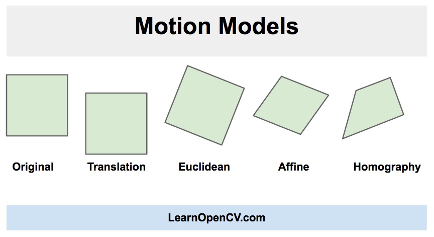
- Homography https://www.learnopencv.com/image-alignment-feature-based-using-opencv-c-python/
Small text:
Homography require template and doc_type
steps:
- Extract features: Commecricla(SURF or SIFT), Free(KAZΑ)
- Match the features (FLANN or BruteForce…) and filter the matchings
- Find the geometrical transformation (RANSAC or LMeds…)
3.25.1. AKAZA
- https://docs.opencv.org/3.4.8/db/d70/tutorial_akaze_matching.html
- https://stackoverflow.com/questions/47496287/how-would-i-use-orb-detector-with-image-homography
- https://docs.opencv.org/2.4/doc/tutorials/features2d/feature_homography/feature_homography.html
- http://www.programmersought.com/article/3078224152/
class KazeCropper:

    def __init__(self, img_orig, nn_match_ratio=0.72):
        if img_orig is None:
            print('Could not open or find the image!')

        height = 674  # average prep
        width = 998  # average
        self.img_orig = img_orig
        if len(img_orig.shape) == 2 or img_orig.shape[2] == 1:
            gray = img_orig
        else:
            gray = cv.cvtColor(img_orig, cv.COLOR_BGR2GRAY)


        gray = imutils.resize(gray, width=width)  # resized
        # CLAHE (Contrast Limited Adaptive Histogram Equalization)
        # clahe = cv.createCLAHE(clipLimit=0.2, tileGridSize=(30,30))
        # clahe.apply(lab_planes[0])

        gray = cv.fastNlMeansDenoising(gray, h=5, templateWindowSize=10)  # denoise
        # cv.imshow('image', self.img_orig)  # show image in window
        # cv.waitKey(0)  # wait for any key indefinitely
        # cv.destroyAllWindows()  # close window q
        self.akaze = cv.AKAZE_create()

        self.kpts2, self.desc2 = self.akaze.detectAndCompute(gray, None)

        self.matcher = cv.DescriptorMatcher_create(cv.DescriptorMatcher_BRUTEFORCE_HAMMING)
        # self.matcher = cv.DescriptorMatcher_create(cv.DescriptorMatcher_BRUTEFORCE_HAMMINGLUT)
        self.nn_match_ratio = nn_match_ratio  # 0.75  # Nearest neighbor matching ratio

    # private
    def transform(self, img, wider: float = 1) -> ():

        kpts1, desc1 = self.akaze.detectAndCompute(img, None)
        # kpts2, desc2 = self.akaze.detectAndCompute(self.img_orig, None)

        nn_matches = self.matcher.knnMatch(desc1, self.desc2, 2)

        matched1 = []
        matched2 = []

        for m, n in nn_matches:
            if m.distance < self.nn_match_ratio * n.distance:
                matched1.append(kpts1[m.queryIdx])
                matched2.append(self.kpts2[m.trainIdx])

        # DEBUG
        # print('A-KAZE Matching Results')
        # print('*******************************')
        # print('# Keypoints 1:                        \t', len(kpts1))
        # print('# Keypoints 2:                        \t', len(self.kpts2))
        # print('# Matches:                            \t', len(matched1))  # must be > 90

        if len(matched1) < 60:
            sys.stderr.write("Error: Not enough matches")
            return None, None, len(matched1)
        # extract the matched keypoints
        src_pts = np.float32([i.pt for i in matched1]).reshape(-1, 1, 2)
        dst_pts = np.float32([i.pt for i in matched2]).reshape(-1, 1, 2)

        # find homography matrix and do perspective transform
        M, mask = cv.findHomography(src_pts, dst_pts, cv.RANSAC, 2)  # 2

        # apply transformation
        img = cv.warpPerspective(img, M, (int(self.img_orig.shape[1] * wider), int(self.img_orig.shape[0] * wider)))

        return img, M, len(matched1)

    # public
    def crop(self, image) -> any:
        """ Double transformation of image to match template

        :param image:
        :return: image
        """
        if image is None or self.img_orig is None:
            sys.stderr.write('Could not open or find the images!')
            return None

        # prepare incoming image
        img = cv.cvtColor(image, cv.COLOR_BGR2GRAY)
        img = cv.fastNlMeansDenoising(img, h=2, templateWindowSize=4)  # denoise
        # Get transformation matrix
        img, m1, mcount = self.transform(img, wider=1.5)
        if mcount < 60:
            return None
        img, m2, mcount = self.transform(img, wider=1)  # no change
        if mcount < 60:
            return None
        # Apply transformation to original image
        img = cv.warpPerspective(image, m1, (int(self.img_orig.shape[1] * 1.5), int(self.img_orig.shape[0] * 1.5)))
        # cv.imshow("found1", img)
        img = cv.warpPerspective(img, m2, (self.img_orig.shape[1], self.img_orig.shape[0]))
        return img

    def match(self, image, k=2) -> int:
        if image is None or self.img_orig is None:
            sys.stderr.write('Could not open or find the images!')
            return 0

        kpts1, desc1 = self.akaze.detectAndCompute(image, None)
        nn_matches = self.matcher.knnMatch(desc1, self.desc2, 2)
        matched1 = []

        for m, n in nn_matches:
            if m.distance < self.nn_match_ratio * n.distance:
                matched1.append(kpts1[m.queryIdx])
        return len(matched1)
3.25.2. findHomography
- может быть полезным https://web-answers.ru/c/python-opencv-ispolzujte-findhomography-i.html
cv.findHomography(src_pts, dst_pts, cv.RANSAC, 5.0)
Normal
- srcPoints -
- dstPoints -
Special
- method -
- 0 - a regular method using all the points
- CV_RANSAC - RANSAC-based robust method
- CV_LMEDS - Least-Median robust method
- ransacReprojThreshold (used in the RANSAC method only) - Maximum allowed reprojection error to treat a point pair as an inlier
- mask: Any = None,
- maxIters: Any = None,
- confidence: Any = None
3.26. Morphological Transformations
https://docs.opencv.org/master/d9/d61/tutorial_py_morphological_ops.html
- Erosion - уменьшить толщину как Convolution
- Dilation - утолщить
- Opening - cv.morphologyEx(img, cv.MORPH_OPEN, kernel) - erosion followed by dilation
- remove noise outside
- find out horizontal or vertical lines
- Clothing - cv.morphologyEx(img, cv.MORPH_CLOSE, kernel) - Dilation followed by Erosion
- to remove small points inside large one
- to group contours
- Morphological Gradient
- Top Hat
- Black Hat
3.27. Deep Neural Network module (dnn)
- Pros:
- легковесности решения
- легче перенос на другие платформы
- упрощает процедуру создания гибридных алгоритмов
- загрузка и запуск моделья - Caffe, TensorFlow или Torch - Поддерживаются все основные слои
- Cons:
- только возможность выполнения прямого прохода (forward pass)
- преобразует модели из различных фреймворков в свое внутреннее представление, возникают вопросы сохранения качества
3.28. USECASES
3.28.1. resize with black are keep ratio
def resize_image(img, size=(28,28)):

    h, w = img.shape[:2]
    c = img.shape[2] if len(img.shape)>2 else 1

    if h == w:
        return cv2.resize(img, size, cv2.INTER_AREA)

    dif = h if h > w else w

    interpolation = cv2.INTER_AREA if dif > (size[0]+size[1])//2 else
                    cv2.INTER_CUBIC

    x_pos = (dif - w)//2
    y_pos = (dif - h)//2

    if len(img.shape) == 2:
        mask = np.zeros((dif, dif), dtype=img.dtype)
        mask[y_pos:y_pos+h, x_pos:x_pos+w] = img[:h, :w]
    else:
        mask = np.zeros((dif, dif, c), dtype=img.dtype)
        mask[y_pos:y_pos+h, x_pos:x_pos+w, :] = img[:h, :w, :]

    return cv2.resize(mask, size, interpolation)
3.28.2. subimage
roi=im[y:y+h,x:x+w]
contours, hierarchy = cv.findContours(img_with_squares, cv.RETR_LIST, cv.CHAIN_APPROX_SIMPLE)
# get rectangle points:
cnt = contours[0]
x,y,w,h = cv.boundingRect(cnt)
roi = img[y:y+h,x:x+w]
3.28.3. scale to target height
def img_to_small(img, height_target=575): # TODO: resize by smallest dimension scale_percent = round(height_target / img.shape[1], 3) width = int(img.shape[1] * scale_percent) height = int(img.shape[0] * scale_percent) dim = (width, height) img_resized = cv.resize(img, dim) return img_resized, scale_percent
3.28.4. colours
- RGB
Y = 0.299 R + 0.587 G + 0.114 B
img = cv2.imread(rgbImageFileName) #BGR default
b1 = img[:,:,0] # Gives **Blue**
b2 = img[:,:,1] # Gives Green
b3 = img[:,:,2] # Gives **Red**
img = cv.cvtColor(img, cv.COLOR_RGB2GRAY)
- visualize HSV range
import numpy as np
import cv2

lower_b = np.array([110,50,50])
upper_b = np.array([130,255,255])

s_gradient = np.ones((500,1), dtype=np.uint8)*np.linspace(lower_b[1], upper_b[1], 500, dtype=np.uint8)
v_gradient = np.rot90(np.ones((500,1), dtype=np.uint8)*np.linspace(lower_b[1], upper_b[1], 500, dtype=np.uint8))
h_array = np.arange(lower_b[0], upper_b[0]+1)

for hue in h_array:
    h = hue*np.ones((500,500), dtype=np.uint8)
    hsv_color = cv2.merge((h, s_gradient, v_gradient))
    rgb_color = cv2.cvtColor(hsv_color, cv2.COLOR_HSV2BGR)
    cv2.imshow('', rgb_color)
    cv2.waitKey(250)

cv2.destroyAllWindows()
- contours to rectanges and draw with numbers
contours, hierarchy = cv.findContours(img_with_squares, cv.RETR_LIST, cv.CHAIN_APPROX_SIMPLE)
    # get rectangle points:
    rects = []
    for cnt in contours:  # cnt = contours[0]
        x, y, w, h = cv.boundingRect(cnt)
        ret.append((x, y, w, h))
for i, rec in enumerate(rects):
        x, y, w, h = rec
        cv.rectangle(img_r, (x, y), (x + w, y + h), color=(0, 255, 0), thickness=2)
        cv.putText(img_r, str(i),
                   org=(x + i * 40, y - 10),
                   fontFace=cv.FONT_HERSHEY_PLAIN,
                   fontScale=3,
                   color=(0, 255, 0),
                   thickness=2)
3.28.5. most common colour
        ntmp = cv2.pyrDown(self.image)
        tmp = cv2.pyrDown(tmp)
        tmp = cv2.pyrDown(tmp)
        tmp = cv2.pyrDown(tmp)
        b, g, r = cv2.split(tmp)
        bc = int(np.bincount(b[0]).argmax())  # most common colours
        gc = int(np.bincount(g[0]).argmax())
        rc = int(np.bincount(r[0]).argmax())
3.28.6. max x min y
minmax_unmodified = np.prod(self.cluster_coords, axis=1)

        minx_miny = np.argmin(minmax_unmodified)  # верхний левый
        maxx_maxy = np.argmax(minmax_unmodified)  # верхний правый

        ccopy = self.cluster_coords.copy()
        ccopy = np.where(ccopy == 0, 0.01, ccopy)  # devide by zero
        ccopy[:, 1] = np.reciprocal(ccopy[:, 1])  # Y^-1, ???????? X/Y
        minx_maxy = np.argmin(np.prod(ccopy, axis=1))

        ccopy = self.cluster_coords.copy()
        ccopy = np.where(ccopy == 0, 0.01, ccopy)
        ccopy[:, 0] = np.reciprocal(ccopy[:, 0])  # X^-1, ???????? Y/X
        maxx_miny = np.argmin(np.prod(ccopy, axis=1))
        # по индексам
        corners = np.rint(self.cluster_coords[[minx_miny, maxx_miny, maxx_maxy, minx_maxy, minx_miny]]).astype(np.int)
3.28.7. Images blending-adding
- gray bitwise
sign = cv.imread(filename, cv.IMREAD_GRAYSCALE)
            sign = 255 - sign
            ret, sign = cv.threshold(sign, 60, 255, cv.THRESH_TOZERO)

            # RANDOM SHIFT SING TODO: random resize
            M = np.float32([[(random.random() + 0.2) * 1.7, 0, random.randint(-70, 70)],
                            [0, (random.random() + 0.2) * 1.7, random.randint(-70, 70)]])
            sign = cv.warpAffine(sign, M, sign.shape)

            cv.imshow('image', sign)  # show image in window
            cv.waitKey(0)  # wait for any key indefinitely
            cv.destroyAllWindows()  # close window

            sign = 255 - sign
            # random brightness
            ret, sign = cv.threshold(sign, random.randint(60, 200), 255, cv.THRESH_TOZERO)
            h = 300
            w = 300
            # random subimage
            alt = random.randint(-280, +50)
            y = random.randint(0, height - h - alt)
            x = random.randint(0, width - w - alt)
            subdoc = doc[y:y + h + alt, x:x + w + alt]
            subdoc = cv.resize(subdoc, dsize=(h, w))
            sign = cv.resize(sign, dsize=(h, w))
            sign_b = sign
            sign = cv.bitwise_and(subdoc, subdoc, mask=sign)
            sign = cv.bitwise_and(sign, sign_b)
3.28.8. filter contours
# contours to points
c_points = []
    for a in contours:
        for aa in a:
            c_points.append([aa[0][0], aa[0][1]])
c_points = np.array(c_points)

# crop image
x, y, w, h = rect
croped = img[y:y + h, x:x + w].copy()

# filter points
        contours, hierarchy = cv2.findContours(thresh, cv2.RETR_TREE, cv2.CHAIN_APPROX_SIMPLE)
        for i in range(len(contours)):
            nxt, prev, first_child, parent = hierarchy[0, i]
            if first_child == -1:  # filter very small
                contours[i] = None
            if nxt == -1 or prev == -1:  # filter very large
                contours[i] = None

        contours = np.array(list(filter(lambda x: x is not None, contours)))  # filter
3.28.9. tables
corner detection vs I suggest you detect the lines instead, e.g. using Hough transform, followed by edge chaining, followed by robust line fitting on each chain.
3.28.10. rotate with PIL and Hough Lines
def rotate_image(img) -> np.array:
    """ HoughLines and PIL used """
    edges = cv.Canny(img, 150, 250, apertureSize=3)
    lines = cv.HoughLinesP(edges, 2, np.pi / 180, 100, minLineLength=300, maxLineGap=10)
    import math

    angles1 = []
    # angles2 = []
    if lines is not None:
        for line in lines:
            x1, y1, x2, y2 = line[0]
            angle = math.atan2(x2 - x1, y2 - y1)
            # print(angle)
            # cv.line(img, (x1, y1), (x2, y2), (0, 255, 0), 2)
            if abs(angle) < 2:
                angles1.append(angle)
            # if abs(angle) > 2:
            #     angles2.append(angle)

        median1_radian = np.median(angles1)
        # median2_radian = np.median(angles1)

        from PIL import Image

        img = cv.cvtColor(img, cv.COLOR_BGR2RGB)
        pil_image: Image.Image = Image.fromarray(img)

        # if len(angles1) > len(angles2):
        mr = median1_radian
        # print(mr)
        # else:
        #     mr = median2_radian
        pil_image = pil_image.rotate(math.degrees(math.pi/2 - mr), Image.NEAREST, fillcolor=(220,220,220))  # nearest not working
        img = np.array(pil_image)
        # Convert RGB to BGR
        img = img[:, :, ::-1].copy()

    return img
3.28.11. PIL convert
OpenCV to PIL Image:
- img = np.array(pil_image)
- # img = img[:, :, ::-1].copy()
3.28.12. rotate
center = (img.shape[1] // 2, img.shape[0] // 2)
scale = 1.03
angle = degree
rot_mat = cv.getRotationMatrix2D(center, angle, scale)
img = cv.warpAffine(img, rot_mat, (img.shape[1], img.shape[0]), borderMode=cv.BORDER_REPLICATE)
3.28.13. resize, shift-translate, shrinking with warpAffine
3.28.14. Lines
- remove vertical horizontal lines
V = cv.Sobel(thresh, cv.CV_8U, dx=1, dy=0) # vertical lines H = cv.Sobel(thresh, cv.CV_8U, dx=0, dy=1) # horizontal lines mask = np.zeros(gray.shape[:2], dtype=np.uint8) contours = cv.findContours(V, cv.RETR_LIST, cv.CHAIN_APPROX_SIMPLE)[1] height = gray.shape[0] for cnt in contours: (x, y, w, h) = cv.boundingRect(cnt)
if h > height / 3 and w < 40: cv.drawContours(mask, [cnt], -1, 255, -1) img2 = cv.resize(mask, (900, 900)) cv.imshow("ROI", img2) cv.waitKey(0) cv.destroyAllWindows() mask = cv.morphologyEx(mask, cv.MORPH_DILATE, None, iterations=3) img2 = cv.resize(mask, (900, 900)) cv.imshow("ROI", img2) cv.waitKey(0) cv.destroyAllWindows() thresh[mask == 255] = 0
- remove small lines
 linek = cv.zeroes((27, 27), dtype=np.uint8)
 linek[..., 13] = 1
 linek[13, ...] = 1
 x = cv.morphologyEx(thresh_save, cv.MORPH_OPEN, linek, iterations=1)
 # or
 cross = cv.getStructuringElement(cv.MORPH_CROSS, (27, 27))
 x = cv.morphologyEx(thresh_save, cv.MORPH_OPEN, cross, iterations=1)
- find out lines (short one) & boxes
# left only vertical lines
vertical_kernel = cv2.getStructuringElement(cv2.MORPH_RECT, (1,15))
vertical = cv2.morphologyEx(img_bin, cv2.MORPH_OPEN, vertical_kernel, iterations=1)

# left only horizontal lines
horizontal_kernel = cv2.getStructuringElement(cv2.MORPH_RECT, (15,1))
horizontal = cv2.morphologyEx(img_bin, cv2.MORPH_OPEN, horizontal_kernel, iterations=1)

# left only this lines
img_opened = cv2.addWeighted(vertical, 0.5, horizontal, 0.5, 0.0)
_, img_opened = cv2.threshold(img_opened, 0, 255, cv2.THRESH_BINARY)

# find out boxes
CANNY_KERNEL_SIZE = 100
img_canny = cv2.Canny(img, CANNY_KERNEL_SIZE, CANNY_KERNEL_SIZE)
3.28.15. minAreaRect
- rect = cv.minAreaRect(save_contour)
- ((196., 471.), (358., 423.), -3.)
- width = int(rect[1][0])
- height = int(rect[1][1])
- rect[0] - center
3.28.16. detect shape of contour
 for c in cnts:
        cv.contourArea(c)
        area = cv.contourArea(c)
        if 1000 < area < 2100:
            peri = cv.arcLength(c, True)
            approx = cv.approxPolyDP(c, 0.04 * peri, True)
            print(area, len(approx)) # len(approx) - vertices
            newc.append(c)
3.28.17. detect objects by shape (link)
3.28.18. image to batch
    im = cv.imread('./train/passport_ranee/_0_353.png')
    im = cv.cvtColor(im, cv.COLOR_BGR2GRAY)
    im = im.reshape(im.shape + (1,))  # channels
    im = im.reshape((1,) + im.shape)  # batches
3.28.19. cut part of image
def get_rectangle(img, rect):
    "extract rectangle and return rectangle image"
    xy1, xy2 = rect
    return img[xy1[1]:xy2[1],xy1[0]:xy2[0],:]
3.29. troubleshooting
error: (-215:Assertion failed) npoints > 0 in function 'drawContours'
4. MMCV
OpenMMLab - company name and platform
- MMEngine - provide universal training and evaluation engine
- MMCV - neural network operators and data transforms, which serves as a foundation of the whole project
provide:
- Image/Video processing
- Image and annotation visualization
- Image transformation
- Various CNN architectures
- High-quality implementation of common CPU and CUDA ops
5. Abby
ABBYY FineReader
- Optical Character Recognition – OCR
- Машинное Обучение на шаблонах документах.
1С Скан-Загрузке документов
распознование качественных сканов без обучения
классификации неструктурированных документов в соответствии задачами организации
6. Rusnarbank_OPENCV
- https://gitlab.rusnarbank.ru/m.smirnov/Rusnarbank_OPENC
- https://www.pyimagesearch.com/2018/08/20/opencv-text-detection-east-text-detector/
- docker-compose build
input: PDF only
MainOpenCV.py
- ScanerFixClass - Class
- HoughCheck() преобразование Хафа (Hough Transform)
- вычисления угла наклона по прямым линиям - self.degree
- выпрямление - imutils - self.image
- TODO: если текст не распознается, перевернуть 180%
- RotatedRectWithMaxArea() - вычисления повернутого прямоугольника с максимальной площадью
- self.RectWithMaxArea
- CropAroundCenter() - отсечения от изображения всего лишнего
- self.image
- DetectBox() - для обрезки белых областей со всех сторон изображения
- детектора границ Canny
- HoughCheck() преобразование Хафа (Hough Transform)
- GetDocumentType - Class
- textboxes = UtilModule.UtilClass.GetText(image) - координаты боксов с текстом
- get_type_by_text()
- вырезаем изображение для каждого бокса
- pytesseract.image_to_string
- ищим текст в каждом боксе, совпал - это такой-то документ, break
- ParserClass - Class
- PageProcessing(image_path) - основная функция
- ScanerFixClass(image)
- GetDocumentType(fix_obj.image)
- ParserClass(image, type) - возвращает return_dict
- MainProcessingClass
- __init__ (file_pdf) создает Redis
- UtilModule.UtilClass.PdfToPng -> fileslist
- PageProcessing(id_img, image_path) -> resilt[id_img] = res
6.1. Redis
один порт, один Redis, несколько workers
6.2. client
import requests
files = {'pdf': open(r"C:\Users\Chepilev_VS\Downloads\Rusnarbank_OPENCV-master\examples\bad\1_2_2018.pdf", 'rb')}
job_id = requests.post("http://localhost:5000/upload", files=files).json()["id"]
result = requests.get("http://localhost:5000/get?id="+job_id).json()
print(result)
6.3. dependences
git+https://github.com/GeorgiyDemo/cv_algorithms.git - OpenCV algorithms are are not available
- OpenCV 3
- ?
git+https://github.com/GeorgiyDemo/UliEngineering.git
- Electronics Engineering ?
redis==3.1.0
- Резидентная NoSQL СУБД
opencv-python==3.4.5.20 imutils==0.5.2
- displaying Matplotlib images easier with OpenCV
- image processing - translation, rotation, resizing, skeletonization
pytesseract==0.2.6 requests==2.21.0 pdf2image==1.4.0 PyYAML==3.13 networkx==2.2 scipy==1.2.0 toolz==0.9.0 rq==0.13.0 sentry-sdk==0.7.10
6.4. tesseract
- debian testing
- apt-get install tesseract-ocr-rus
- /usr/share/tesseract-ocr/4.00/tessdata/rus.traineddata
6.5. Return JSON
- MainOpenCV.py:323 {'1':('1', OUTPUT_OBJ)}
- OKUD.py OKUD_0710001 class init -> 240 -> 217 -> 111
- MatrixToJson.py:104 ToJSON class - property JSON -> 272
- SmallTableProcessing() - 'info': self.small_table в основном self.JSON
- суммируем в Processing() or FiveDocProcessing()(для продолжения листа)
- self.JSON = {'qc': 2, 'document_type': '1', "period": [matrix]}
- данные основной таблицы matrix:
- столбцы по датам {'31122016': {'hindex': 5, 'codes': []}}
- hindex - номер столбца от левого края, начиная с какого - хз
- codes -
- столбцы по датам {'31122016': {'hindex': 5, 'codes': []}}
JSON - { "status": "ready", "pages": [OUTPUT_OBJ, OUTPUT_OBJ ….] }
where OUTPUT_OBJ = {"qc":0, } л
Успешные ответы
- {"status": "ready", "pages": "…"} - первый ответ get
7. passport
rec:
- https://www.pyimagesearch.com/2015/11/30/detecting-machine-readable-zones-in-passport-images/
- https://habr.com/ru/post/208090/
colour:
- http://www.compvision.ru/forum/index.php?/topic/1568-%D1%80%D0%B0%D1%81%D0%BF%D0%BE%D0%B7%D0%BD%D0%B0%D0%B2%D0%B0%D0%BD%D0%B8%D0%B5-%D1%82%D0%B5%D0%BA%D1%81%D1%82%D0%B0-%D0%BF%D0%B0%D1%81%D0%BF%D0%BE%D1%80%D1%82%D0%B0-opencv/
- automatic adj for OCR https://stackoverflow.com/questions/56905592/automatic-contrast-and-brightness-adjustment-of-a-color-photo-of-a-sheet-of-pape
rectangle:
- https://stackoverflow.com/questions/26583649/opencv-c-rectangle-detection-which-has-irregular-side
- OpenCV shape detection https://www.pyimagesearch.com/2016/02/08/opencv-shape-detection/
- https://robotclass.ru/tutorials/opencv-detect-rectangle-angle/
- https://towardsdatascience.com/object-detection-with-neural-networks-a4e2c46b4491
- https://github.com/jrieke/shape-detection
- MRZ https://web.archive.org/web/20140801191250/http://www.fms.gov.ru/upload/iblock/fe3/prikaz_mchz279.pdf
- https://github.com/Shreeshrii/tessdata_ocrb
- Машиночитаемая запись МЧЗ
- двух строк по 44 символа
- Шрифт OCR-B type 1 (Стандарт ИСО 1073/II).
- верхняя строка 6-44 модернизированный клер
- 10, 20, 28, 43, 44 нижней строки МЧЗ содержат контрольные цифры.
- top
- 1-2 PN Passport National - Тип документа
- 3-5 RUS - код ИКАО
- 6-44 BAQRAMOV<<AMIR<IL9GAM<<0GLY<<<<<<<<<<<< - БАЙРАМОВ \n АМИР \n ИЛЬГАМ - ОГЛЫ
- дефис = '<' - знак заполнитель
- имя сокращается на букве, которая является 42 знаком строки, знака-заполнителя вносится первая буква отчества.
- фамилия сокращается на букве, которая является 39 знаком строки, после двух знаков-заполнителей последовательно вносятся первая буква имени, знак-заполнитель, первая буква отчества
- bottom
- 1-9 460123456 - серии 4601 № 123456
- 10 Контрольная цифра - по 1-9
- 11-13 RUS
- 14-19 YYMMDD 931207 - 1993.12.07 - Дата рождения
- 20 Контрольная цифра - по 14-19
- 21 F or M - женский, мужской
- 22-27 Дата истечения срока действия или все <, вместе с контрольной ццифрой
- 28 Контрольная цифра or <
- 29 Последняя цифра серии
- 30-35 YYMMDD Дата выдачи паспорта
- 36-41 Код подразделения
- 42 < в контрольной сумме учитывается как 0
- 43 Контрольная цифра 29-42
- 44 Контрольная цифра 1-10, 14-20, 22-28, 29-43
7.1. error
rq.worker:opencv-tasks: file (7120f9a5-7fde-41ba-96f4-ef1da72c5c1d)
Traceback (most recent call last):
return method_number_list[method_number](obj).OUTPUT_OBJ
File "/code/parsers/multiparser.py", line 22, in passport_and_drivelicense
aop = passport_main_page(img_cropped)
File "/code/parsers/passport.py", line 162, in passport_main_page
res_i = fio_checker.double_query_name(anonymous_return.OUTPUT_OBJ['MRZ']['mrz_i'], i_pass)
File "/code/groonga.py", line 248, in double_query_name
return FIOChecker._get_appropriate(items1, word1)
File "/code/groonga.py", line 236, in _double_query
equal = [x for x in items if x[2] = 4] # score
File "/code/groonga.py", line 129, in <listcomp>
ERROR:root:Uncatched exception in ParserClass
return self._double_query(word1, word2, self.names_table)
File "/code/groonga.py", line 129, in _get_appropriate
equal = [x for x in items if x[2] = 4] # score
KeyError: 2
File "/code/MainOpenCV.py", line 40, in parser_call
7.2. Расчет контрольной суммы
| data | 5 1 0 5 0 9 |
| weight | 7 3 1 7 3 1 |
| after multiply | 35 3 0 35 0 9 |
- Сумма результатов 35 + 3 + 0 + 35 +0 +9 = 82
- 82 / 10 =8, остаток деления 2
- 2
- 361753650
import numpy as np
a=np.array([3,6,1,7,5,3,6,5,0])
b=np.array([7,3,1,7,3,1,7,3,1])
np.sum(a*b)%10
7.3. passport serial number
- http://ukrainian-passport.com/blog/everything-you-have-to-know-about-the-russian-passport/
- consists of two signs and refers to the code assigned to the appropriate area (region) of the Russian Federation.
- indicates the year of passport issue
- passport serial number - six signs
7.4. string metric for measuring the difference between two sequences
- коэффициент Танимото https://grishaev.me/2012/10/05/1/
- https://habr.com/en/post/341148/
8. captcha
8.1. captcha image
8.2. audio capcha
speech recognition model
8.2.1. split audio file by worlds(librosa)
import librosa
import numpy as np
from typing import List
# own
from utils import Captcha

ALPHABET = ('2', '4', '5', '6', '7', '8', '9', 'б', 'в', 'г', 'д', 'ж', 'к', 'л', 'м', 'н', 'п', 'р', 'с', 'т')
ALPHABET_FEATURE = [105.0, 160.0, 74.0, 76.0, 94.0, 146.0, 148.0, 86.0, 106.0, 92.0, 90.0, 83.0, 91.0, 99.0, 104.0, 96.0, 87.0, 79.0, 65.0, 87.0]
FEATURE_RMS_T = 0.093
FEATURE_RMS_P = 0.086


def splitbysilence(y):
    td = 18.2
    hop_length = 9
    intervals = librosa.effects.split(y, top_db=td, hop_length=hop_length)
    pieces = []
    for iv in intervals:
        p = y[iv[0]:iv[1]]
        pa, _ = librosa.effects.trim(p, ref=0.45, top_db=20, hop_length=3)
        pieces.append(pa)
    return pieces


def get_alpha_by_feature(f: float or List[float]) -> str:
    global ALPHABET, ALPHABET_FEATURE
    if isinstance(f, float):
        return ALPHABET[ALPHABET_FEATURE.index(f)]
    else:
        a = [ALPHABET[ALPHABET_FEATURE.index(fi)] for fi in f]
        return ''.join(a)


def calc_feature(sound: np.ndarray, sr):
    f_d = librosa.get_duration(y=sound)
    f_mfcc = np.mean(librosa.feature.mfcc(y=sound, sr=sr, n_fft=100, n_mfcc=20))
    f_2 = np.median(librosa.feature.rms(y=sound, hop_length=100))
    return (abs(f_mfcc) + f_d*1000 + f_2*800)//4   # 4 is enough


def calc_features(c: Captcha or str) -> List[int] or int:
    """ c file math """
    if isinstance(c, Captcha):
        y, sr = librosa.load(c.filepath)
    else:
        y, sr = librosa.load(c)
    split = splitbysilence(y)
    return [calc_feature(sound, sr) for sound in split]


def max_db(y, n_fft=2048):
    s = librosa.stft(y, n_fft=n_fft, hop_length=n_fft // 2)
    d = librosa.amplitude_to_db(np.abs(s), ref=np.max)
    return np.max(abs(d))


def get_alpphabet_feature(alphabet: str or list, captchas_solved: List[Captcha]):
    """ alpha_features = get_alpphabet_feature(ALPHABET, captchas) """
    features = []
    for a in alphabet:
        for c in captchas_solved:
            if a in c.salvation:
                y, sr = librosa.load(c.filepath)
                pieces = splitbysilence(y)
                position = c.salvation.index(a)
                sound: np.ndarray = pieces[position]
                f = calc_feature(sound, sr)
                features.append(f)
                break
    assert len(features) == len(alphabet)
    return features


def audio_decode(file_patch: str) -> str:
    y, sr = librosa.load(file_patch)
    yl = splitbysilence(y)
    features: list = [calc_feature(sound, sr) for sound in yl]
    sol = get_alpha_by_feature(features)
    for i, ch in enumerate(sol):
        if 'п' == ch or 'т' == ch:
            sol_l = list(sol)
            f = np.median(librosa.feature.rms(y=yl[i], hop_length=100))
            if round(float(f), 3) == FEATURE_RMS_P:
                sol_l[i] = 'п'
            elif round(float(f), 3) == FEATURE_RMS_T:
                sol_l[i] = 'т'
            sol = ''.join(sol_l)
    return sol
8.3. reCAPTCHA google
- Version 2 ~2013, also asked users to decipher text or match images if the analysis of cookies and canvas
rendering suggested the page was being downloaded automatically.
- behavioral analysis of the browser's interactions to predict whether the user was a human or a bot
- version 3, at the end of 2019, reCAPTCHA will never interrupt users and is intended to run automatically when users load pages or click buttons.
On May 26, 2012, Adam, C-P and Jeffball - accuracy rate of 99.1% analyse the audio version of reCAPTCHA
- after: the audio version was increased in length from 8 seconds to 30 seconds, and is much more difficult to understand, both for humans as well as bots.
- after: 60.95% and 59.4% respectively
9. optical label
- QRCode origian work - Yue Liu, Ju Yang, Mingjun Liu, “Recognition of QR Code with mobile phones,” Control and Decision Conference, CCDC 2008. Chinese, pp. 203 - 206, 2-4 July 2008. https://www.scribd.com/document/79038295/Recognition-of-QR-Code-With-Mobile-Phones
types https://en.wikipedia.org/wiki/Barcode
- FonCode https://arxiv.org/pdf/1707.09418v1.pdf
- 2d barcode comparision https://medium.com/dynamsoft/what-is-the-difference-between-qr-code-pdf417-and-datamatrix-39f4db881388
- Data Matrix vs QR Code https://www.laserax.com/blog/data-matrix-vs-qr-codes
- barcode and error correction http://www.labelingnews.com/2012/12/barcodes-and-error-correction/
- Data Matrix quality verification accordance with ISO/IEC 15416 http://www.datamatrixcode.net/data-matrix-code-quality-verification/
- Data Matrix NN https://www.researchgate.net/publication/341220437_Detection_of_Data_Matrix_Encoded_Landmarks_in_Unstructured_Environments_using_Deep_Learning
- detect data matrix https://github.com/NaturalHistoryMuseum/gouda/
- generators https://blog.jonasneubert.com/2019/01/23/barcode-generation-python/
- Best Practives https://www.codeproject.com/Articles/20940/Using-Barcodes-in-Documents-Best-Practices
9.1. opencv
opencv 4.x new https://stackoverflow.com/questions/53906178/how-opencv-4-x-api-is-different-from-previous-version
install from source opencv https://docs.opencv.org/3.4.11/d2/de6/tutorial_py_setup_in_ubuntu.html
9.2. qrcode
https://github.com/lincolnloop/python-qrcode
import qrcode img = qrcode.make('Some data here') img.save('path')
9.3. segno
10. OCR ICR
10.1. terms
- handprinted text - characters are written separately, is not about “cursive handwriting”
- handwriting
10.2. Components:
- optical character recognition (OCR) for machine print
- optical mark reading (OMR) for check/mark sense boxes
- bar code recognition (BCR) for barcodes
- and intelligent character recognition (ICR) for hand print.
- MICR – Magnetic ink character recognition
10.3. optical character recognition (OCR)
10.4. intelligent character recognition (ICR)
recognizes different handwriting styles and fonts to intelligently interpret data on forms and physical documents
use of continuously improving algorithms to collect more information about the variances in hand-printed characters and more precisely identify them.
intelligent word recognition (IWR) focuses on reading a word in context rather than recognizing individual characters. is optimized for processing real-world documents that contain mostly free-form, hard-to-recognize data fields that are inherently unsuitable for ICR. (evolved version of ICR)
Robotic Process Automation (RPA) is a technique that automates the configuration of Intelligent character recognition software and ensures that operations are completed without errors.
10.5. Forms processing
hard copy data is filled out by humans and then "captured" from their respective fields
- information entered into data fields
- map of the document, detailing where the data fields are located within the form or document
steps
Assessment of the form structure - to analyze the type of form. Types of forms:
- Fixed forms - data always found
- Semi-structured (or unstructured) form - the location of the data and fields holding the data vary from
document to document. Ex: letters, contracts, and invoices.
11. подпись signature (ˈsɪɡnətʃər;) handwritten
- 2017 SigNet: Convolutional Siamese Network for Writer Independent Offline SignatureVerification https://arxiv.org/pdf/1707.02131.pdf
- https://en.wikipedia.org/wiki/Signature_recognition
- https://ru.qaz.wiki/wiki/Handwriting_recognition
- Wet signatures - person's name written in their own hand with ink (чернилами)
- Biometric Signature == handwritten signature
- forged - подделанный
- offline signature verification or static
- Почерковедческая экспертиза ( Верификация подписи)
- «Подпись» — это собственноручное написание лицом собственной фамилии, имени, инициалов или их частей (элементов), как правило содержащее индивидуальные особенности, позволяющие визуально отличить подпись одного человека от подписи другого.
- «роспись» применяется для подтверждения факта ознакомления работника с какой-либо информацией или документом, уже составленным и подписанным другими лицами.
- http://irsit.ru/files/article/199.pdf
- https://cyberleninka.ru/article/n/algoritmy-verefikatsii-rukopisnyh-podpisey-na-osnove-neyronnyh-setey
- electronic signature https://www.mobbeel.com/en/blog/eidas-types-of-electronic-signature-biometric-signature/
11.1. soft
- abby
12. 12 лучших репозиториев GitHub по компьютерному зрению
Список из наиболее важных Awesome репозиториев GitHub, посвященных компьютерному зрению, которые охватывают широкий спектр исследовательских и образовательных тем. Огромный кладезь знаний из области CV.
- Awesome Computer Vision https://github.com/jbhuang0604/awesome-computer-vision
- Computer Vision Tutorials by Roboflow https://github.com/roboflow/notebooks
- Transformer in Vision https://github.com/Yangzhangcst/Transformer-in-Computer-Vision
- Awesome Referring Image Segmentation https://github.com/MarkMoHR/Awesome-Referring-Image-Segmentation
- Awesome Vision Language Pretraining Papers https://github.com/yuewang-cuhk/awesome-vision-language-pretraining-papers
- Awesome Vision and Language
- Awesome Temporal Action Detection
- Awesome Masked Autoencoders
- Awesome Visual Transformer
- Transformer-Based Visual Segmentation https://github.com/lxtGH/Awesome-Segmentation-With-Transformer
- CVPR 2023 Paper with Code https://github.com/amusi/CVPR2023-Papers-with-Code
- Awesome Deepfakes Detection https://github.com/Daisy-Zhang/Awesome-Deepfakes-Detec
13. VR
за счёт иммерсивных устройств, таких как знакомые всем VR-очки. Очки отслеживают вращение головы.
- Dop: перчатки, наушники, генераторы запахов.
projects:
- Google Street View от Google Maps
- Half-Life: Alyx.
дополненная (AR), смешанная (MR) и расширенная (XR)
Популярные метавселенные:
14. NEXT LEVEL
self-supervised learning, vision transformers, unsupervised object detection, CLIP based text-image scoring, VQA